Chapter 2 Statistics, Probabilities and Matrix Algebra Preliminaries

In the first part of this chapter, we reviewed some concepts and methods in statistics, probability and matrix algebra, which are supposed to be known before taking the class. In the second part, we’ll introduce something new, such as random fields and their related properties.

2.1 Matrix Algebra

Refer to the supplementary materials “supplementary-linear algebra.pdf”.

2.2 Multivariate Gaussian Distribution

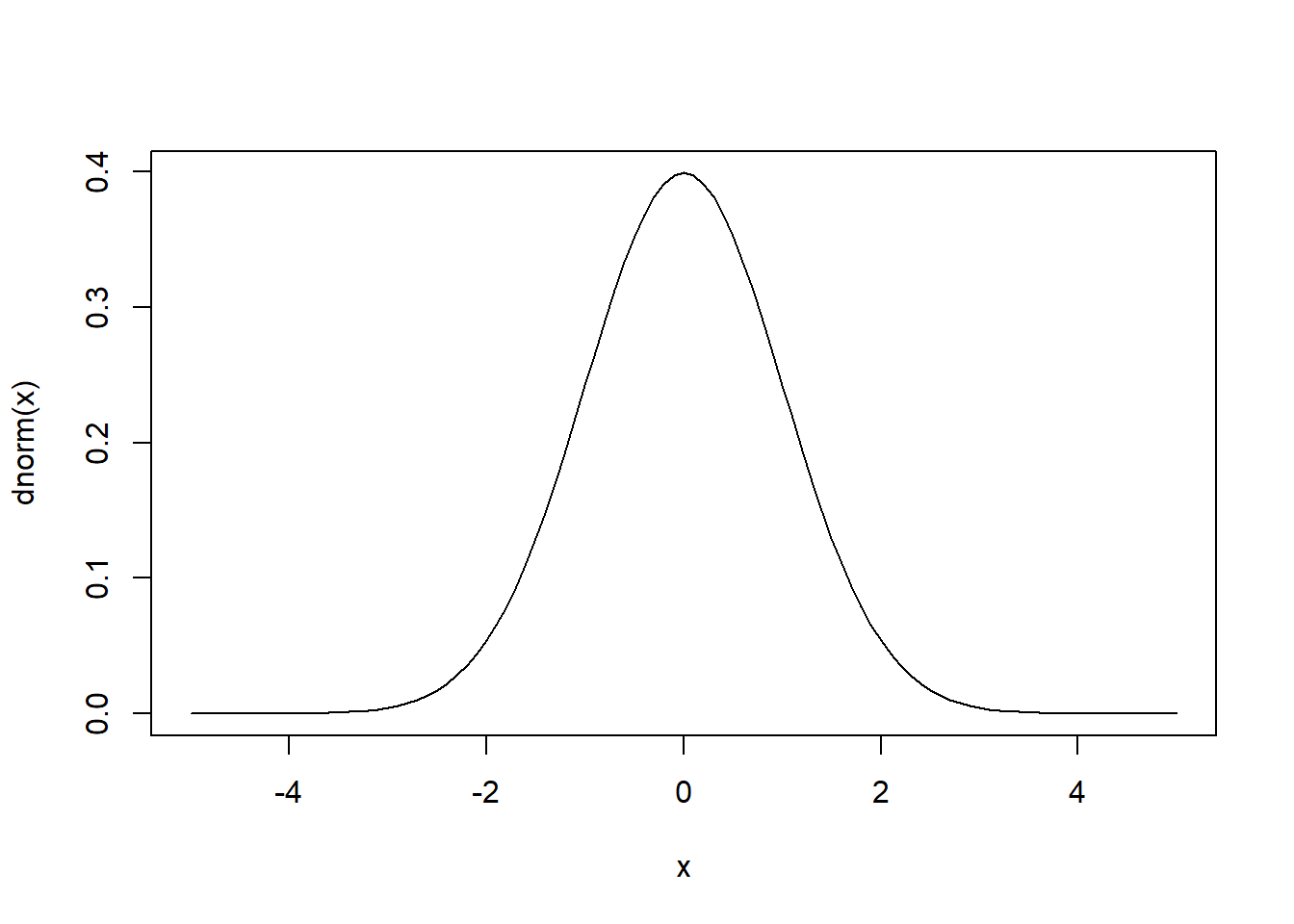
A real valued Gaussian random variable \(X\) (also called normal random variable) with mean \(\mu\) and variance \(\sigma^2\) has the following density function \[f(x) = \frac{1}{\sqrt{2\pi}\sigma} e^{-\frac{(x-\mu)^2}{2\sigma^2}}.\] Usually, it is denoted by \(X\sim N(\mu, \sigma^2)\). For example, the density plot of a Gaussian random variable with mean zero and variance \(1\) is

Now suppose that we have \(n\) independent Gaussian random variables \(X_1,...,X_n\) with \(X_i \sim N(\mu_i, \sigma_i^2).\) Let \({\mathbf{X}}= (X_1,...,X_n)^\top\). Then the joint density of \({\mathbf{X}}\) is just multiplication of densities of \(X_i\)s, that is \[f_{{\mathbf{X}}}(x_1,...,x_n) = (2\pi)^{-n/2}\prod_{i=1}^n \sigma_i^{-1}\exp\left\{-\sum_{i=1}^n \frac{(x_i-\mu_i)^2}{2\sigma_i^2}\right\}.\] But in the real world, most of time \(X_1,...,X_n\) are correlated with each other, which could be generated by \({\mathbf{X}}= {\mathbf{A}}{\mathbf{e}}\) where \({\mathbf{A}}\) is a \(n\times n\) matrix and \({\mathbf{e}}\) are independent Gaussian random vector. So we need to generalize the Gaussian distribution to multivariate case with dependence among components. Here is the definition.

Definition 2.1 (Multivariate Gaussian) A random vector \({\mathbf{X}}=(X_1,...,X_n)^\top\) with mean \({\boldsymbol{\mu}}=(\mu_i)_{i=1}^n\) and variance \(\Sigma=(\sigma_{ij})_{i,j=1}^n\) is said to follow multivariate Gaussian distribution if its density is given by \[f({\mathbf{x}}) = (2\pi)^{-n/2}|\Sigma|^{-1/2}e^{-\frac{1}{2}({\mathbf{x}}-{\boldsymbol{\mu}})^\top \Sigma^{-1}({\mathbf{x}}-{\boldsymbol{\mu}})}, \ \text{for any}\ {\mathbf{x}}=(x_1,...,x_n)^\top\in {\mathbb{R}}^n.\]

Theorem 2.1 There exists a \(n\) dimensional independent Gaussian vector \({\mathbf{e}}\) with mean \({\boldsymbol{\mu}}\) and identity variance \({\mathbf{I}}\) such that the Gaussian random vector \({\mathbf{X}}\) can be represented as \[{\mathbf{X}}= {\mathbf{L}}{\mathbf{e}}+ {\boldsymbol{\mu}},\] where \({\mathbf{L}}\) is the lower triangular matrix in the cholesky decompostion of \(\Sigma\): \(\Sigma = {\mathbf{L}}{\mathbf{L}}^\top\) and \({\boldsymbol{\mu}}\) is the mean of \({\mathbf{X}}\).

Example 2.1 (Bivariate Gaussian density plot) We provide the density plot of a bivariate Gaussian random vector with mean \({\boldsymbol{\mu}}= (0,0)^\top\) and variance \[\Sigma = \begin{pmatrix} 1 & \rho\\ \rho & 1 \end{pmatrix}.\]

2.3 Generalized/Ordinary Least Squares

Let \({\mathbf{Y}}=(y_1,...,y_n)^\top\), \({\boldsymbol{\beta}}=(\beta_1,...,\beta_p)^\top\), \({\boldsymbol{\epsilon}}=(\epsilon_1,...,\epsilon_n)^\top\) and \[{\mathbf{X}}= \begin{pmatrix} x_{11} & x_{12} &\cdots & x_{1p}\\ x_{21} & x_{22} & \cdots & x_{2p}\\ \vdots & \vdots & \cdots & \vdots\\ x_{n1} & x_{n2} &\cdots & x_{np}\\ \end{pmatrix}\]

Consider the following linear model \[\begin{align} \mathbf{Y} = \mathbf{X} \boldsymbol{\beta} + \boldsymbol{\epsilon}, \tag{2.1} \end{align}\]

where \({\mathbb{E}}({\boldsymbol{\epsilon}}) = \mathbf{0}\) and \(\text{Var}({\boldsymbol{\epsilon}}) = \Sigma\).

• Suppose that \(y_i\)s are independent with common variance, then the residual variance \(\text{Var}({\boldsymbol{\epsilon}}) = \sigma^2 {\mathbf{I}}\). In this case, the best linear unbiased estimator of \({\boldsymbol{\beta}}\) is the ordinary least squares estimator, \[\hat {\boldsymbol{\beta}}_{OLS}= ({\mathbf{X}}^\top {\mathbf{X}})^{-1}{\mathbf{X}}^\top {\mathbf{Y}},\] which is obtained by minimizing \[\min_{{\boldsymbol{\beta}}} ({\mathbf{Y}}-{\mathbf{X}}{\boldsymbol{\beta}})^\top ({\mathbf{Y}}-{\mathbf{X}}{\boldsymbol{\beta}}).\]

• Suppose that \(y_i\)s are correlated but with common variance, specifically, \(\text{Var}({\boldsymbol{\epsilon}}) = \Sigma\). In this case, what is the BLUE of \({\boldsymbol{\beta}}\)?

Perform the cholesky decomposition of \(\Sigma\): \(\Sigma = {\mathbf{L}}{\mathbf{L}}^\top\). There exists an \(n\)-dimensional independent random vector \({\mathbf{e}}\) such that \({\boldsymbol{\epsilon}}= {\mathbf{L}}{\mathbf{e}}\). Then the above linear model can be transformed to \[{\mathbf{L}}^{-1}{\mathbf{Y}}= {\mathbf{L}}^{-1}{\mathbf{X}}{\boldsymbol{\beta}}+ {\mathbf{e}}.\] Since \(\text{Var}({\mathbf{e}}) = {\mathbf{I}}\), the BLUE of \({\boldsymbol{\beta}}\) is OLS, that is \[ \hat{\boldsymbol{\beta}}_{GLS} = (({\mathbf{L}}^{-1}{\mathbf{X}})^\top({\mathbf{L}}^{-1}{\mathbf{X}}))^{-1}({\mathbf{L}}^{-1}{\mathbf{X}})^\top {\mathbf{L}}^{-1}{\mathbf{Y}}= ({\mathbf{X}}^\top \Sigma^{-1}{\mathbf{X}})^{-1}{\mathbf{X}}^\top \Sigma^{-1}{\mathbf{Y}}. \] \(\hat{\boldsymbol{\beta}}_{GLS}\) is called the generalized least squares (GLS) estimator of \({\boldsymbol{\beta}}\).

The variance of GLS estimator is \[\text{Var}(\hat{\boldsymbol{\beta}}_{GLS}) = ({\mathbf{X}}^\top \Sigma^{-1}{\mathbf{X}})^{-1}.\]

In the real application, usually the covariance \(\Sigma\) is unknown. We have to model the covariance and get its estimator \(\hat \Sigma\) first. Then \(\hat{\boldsymbol{\beta}}_{GLS}\) is obtained by plugging in \(\hat \Sigma\) to the above formula.

2.4 Maximum Likelihood Estimations

Maximum likelihood estimations (MLE) are often used to estimate parametric models. Here, we still consider the linear model in (2.1). Let \({\boldsymbol{\theta}}=(\theta_1,...,\theta_q)^\top \in \Theta\) where \(\Theta\) is the parameter space. Suppose that the covariance \(\Sigma\) is a function of \({\boldsymbol{\theta}}\). We use the notation \(\Sigma({\boldsymbol{\theta}})\) to represent it. To apply MLE, we need know the distribution of \({\mathbf{Y}}\). Here, we assume \({\mathbf{Y}}\) follows multivariate Gaussian distribution. Then the MLE of \({\boldsymbol{\beta}}\) is obtained by maximizing the log likelihood function, \[\log \ell({\boldsymbol{\beta}},{\boldsymbol{\theta}}; {\mathbf{Y}}) = -\frac{n}{2}\log(2\pi)-\frac{1}{2}\log|\Sigma({\boldsymbol{\theta}})| - \frac{1}{2}({\mathbf{Y}}-{\mathbf{X}}{\boldsymbol{\beta}})^\top \Sigma^{-1}({\boldsymbol{\theta}})({\mathbf{Y}}-{\mathbf{X}}{\boldsymbol{\beta}}).\] For any fixed \({\boldsymbol{\theta}}\in \Theta\), the unique \({\boldsymbol{\beta}}\) that maximize \(\log \ell({\boldsymbol{\beta}},{\boldsymbol{\theta}};{\mathbf{Y}})\) is \[\hat {\boldsymbol{\beta}}_{MLE} = ({\mathbf{X}}^\top \Sigma^{-1}({\boldsymbol{\theta}}){\mathbf{X}})^{-1}{\mathbf{X}}^\top \Sigma^{-1}({\boldsymbol{\theta}}){\mathbf{Y}},\] which would be the GLS estimator of \({\boldsymbol{\beta}}\) when \(\Sigma(\theta)\) is the actual variance of \({\mathbf{Y}}\).

Plugging \(\hat {\boldsymbol{\beta}}_{MLE}\) to \(\log \ell({\boldsymbol{\beta}},{\boldsymbol{\theta}}; {\mathbf{Y}})\), we obtain \[L({\boldsymbol{\theta}}; {\mathbf{Y}}) = -\frac{1}{2}\log|\Sigma({\boldsymbol{\theta}})| -\frac{1}{2}{\mathbf{Y}}^\top\left\{\Sigma^{-1}({\boldsymbol{\theta}})-\Sigma^{-1}({\boldsymbol{\theta}}){\mathbf{X}}({\mathbf{X}}^\top \Sigma^{-1}({\boldsymbol{\theta}}){\mathbf{X}})^{-1}{\mathbf{X}}^\top \Sigma^{-1}({\boldsymbol{\theta}})\right\}{\mathbf{Y}}.\] \(\hat {\boldsymbol{\theta}}_{MLE}\) can be obtained by maximizing \(L({\boldsymbol{\theta}};{\mathbf{Y}})\). Most of time there is no closed-form solution. In general, it is obtained with numerical methods.

2.5 Random Fields for spatial models

In a statistical analysis, we usually try to model the data by a probabilistic model. As a very simple example, suppose that we randomly selected \(n\) adults in US and measured their heights, say \(x_1,...,x_n\). We usually model the height of an adult as a random variable \(X\) with mean \(\mu\) and \(\sigma^2\). Let \(F(\cdot)\) be the distribution of \(X\). Usually, it is assumed to be Gaussian distribution. Then we develop statistical methods to estimate the mean, variance, or even the distribution \(F\) if it is unknown. Here, any data point is considered as a possible outcome of \(X\) and is generated by random sampling. In other words, the probabilistic model provides the data generation mechanism.

Now consider the case for spatial data. What kind of probabilistic model shall we use? Suppose that we observed temperatures at locations \({\mathbf{s}}_1, ..., {\mathbf{s}}_n\) inside a region \(\mathcal{D}\) at time \(t\), say \(y({\mathbf{s}}_1),...,y({\mathbf{s}}_n)\). We would like to predict temperatures at other locations in \(\mathcal{D}\).

Here is a reasonable idea. Prior to time \(t\), the temperature of any point in \(\mathcal{D}\), say \(Y({\mathbf{s}})\), could be considered as a continuous random variable with potential probability to take any possible value. And hence the temperatures for all points in \(\mathcal{D}\) can be modeled as a random surface. All possible \(3D\) surfaces can be considered as the sample space \(\mathcal{S}\). The temperatures at time \(t\) would be one \(3D\) surface out of \(\mathcal{S}\). In order to measure the uncertainty, we should also model the distribution of any events in the sample space \(\mathcal{S}\). Further, at time \(t\), we have \(n\) observations of the potential surface for \(Y\). To predict \(Y\)s at other locations, we should consider the distribution of those \(3D\) surfaces in \(\mathcal{S}\) whose values at \({\mathbf{s}}_1,...,{\mathbf{s}}_n\) are fixed, that are \(y({\mathbf{s}}_1),...,y({\mathbf{s}}_n)\).

A probability tool to implement the above modeling idea is called random process, that is a collection of random variables on a given index set \(\mathcal{D}\), say \(Y=\{Y({\mathbf{s}}), {\mathbf{s}}\in \mathcal{D}\}\). Here, the domain \(\mathcal{D}\) could be discrete, continuous, finite or infinite. If \(\mathcal{D}\) is a domain in Euclidean space with dimension greater than one, \(Y\) is called random field. Since spatial data are usually collected in \(2D\) or \(3D\) domain, we’ll use the name “random field” rather than “random process” in the following even if the data were collected in \(1D\) domain.

How do we define the distribution of a random field, since its potential value is a curve or a surface? That would be a probability measure defined on a functional space, which is abstract and beyond the scope of our class. Rather, we would consider a family of finite dimensional distribution functions (F.D.D.), that are for any \(n\) and any \({\mathbf{s}}_1,...,{\mathbf{s}}_n \in \mathcal{D}\), the distribution of \(Y({\mathbf{s}}_1),...,Y({\mathbf{s}}_n)\) is modeled by \[F(y_1,...,y_n) = \mathbb{P}(Y({\mathbf{s}}_1) < y_1,...,Y({\mathbf{s}}_n) < y_n),\] where \(F\) is a family of well-defined functions on any finite dimensional space \(\mathbb{R}^d\). By Kolmogorov Consistency Theorem, the family of F.D.D. will uniquely determine the probability measure of a stochastic process.

The F.D.D. are sufficient for most of estimation and prediction problems in spatial analysis. Hence, most of time we do not need to characterize the probability measure of the whole process, especially in applications.

A very popular model in spatial statistics is Gaussian random field, which is a random field whose F.D.D. is a multivariate Gaussian distribution, that is \[\mathbb{P}(Y({\mathbf{s}}_1) < y_1,...,Y({\mathbf{s}}_n) < y_n) =\int_{-\infty}^{y_1}\cdots\int_{-\infty}^{y_n} (2\pi)^{-n/2}|\Sigma|^{-1/2}e^{-\frac{1}{2}({\mathbf{x}}-{\boldsymbol{\mu}})^\top \Sigma^{-1}({\mathbf{x}}-{\boldsymbol{\mu}})}d{\mathbf{x}},\] where \({\mathbf{x}}=(x_1,...,x_n)^\top\), \({\boldsymbol{\mu}}\) is a vector representing the mean of \(Y\) at locations \({\mathbf{s}}_1,...,{\mathbf{s}}_n\) and \(\Sigma\) is the covariance matrix of \((Y({\mathbf{s}}_1),...,Y({\mathbf{s}}_n))^\top\).

From above we can see that a Gaussian random field should have a well-defined mean function \(\{\mu({\mathbf{s}}),{\mathbf{s}}\in \mathcal{D}\}\) and a valid covariance function \(C({\mathbf{s}},{\mathbf{s}}')\) for any \({\mathbf{s}},{\mathbf{s}}'\in\mathcal{D}\).

As is well known, the distribution of a Gaussian random variable is determined by its mean and variance. From above definition, the distribution of a Gaussian random field is determined by its mean function \(\mu({\mathbf{s}})\) and covariance function \(C({\mathbf{s}},{\mathbf{s}}')\).

In general, there is usually no restriction for the mean function \(\mu({\mathbf{s}})\). However, for a non-degenerate random field, the covariance function \(C({\mathbf{s}},{\mathbf{s}}')\) should be positive definite, that is given fixed \(n\), for any \({\mathbf{s}}_1,...,{\mathbf{s}}_n\in \mathcal{D}\) and any \(a_1,...,a_n\), \[\sum_{i,j=1}^n a_ia_jC({\mathbf{s}}_i,{\mathbf{s}}_j) \geq 0,\] where the above equality only holds when \(a_1=\cdots=a_n=0\). Indeed, this follows from \[\sum_{i,j=1}^n a_ia_jC({\mathbf{s}}_i,{\mathbf{s}}_j) =\text{Var}\left(\sum_{i=1}^n a_iY({\mathbf{s}}_i)\right)\geq 0.\]

Example 2.2 (Simulated Gaussian random fields) We simulated a Gaussian random field in \([-3,3]^2\) with mean zero and exponential covariance function \(C({\mathbf{s}},{\mathbf{s}}')= \exp(-0.5|{\mathbf{s}}-{\mathbf{s}}'|)\).

Summary:

1. A random field model is appropriate to model spatial data, among which, Gaussian random fields are the most popular models in spatial statistics.

2. The distribution of a random field is determined by its finite dimensional distributions (F.D.D.). For a Gaussian random field, the finite dimensional distributions are multivariate Gaussian distributions.

3. The mean of a random field is a function defined on the domain \(\mathcal{D}\), say \(\mu({\mathbf{s}}),{\mathbf{s}}\in\mathcal{D}\); the variance of a random field is a function defined on the product space \(\mathcal{D}\times \mathcal{D}\), say \(C({\mathbf{s}},{\mathbf{s}}'), {\mathbf{s}},{\mathbf{s}}'\in \mathcal{D}\). The distribution of a Gaussian random field is determined by its mean function and covariance function.

4. Only positive definite function on \(\mathcal{D}\times \mathcal{D}\) can be used to model the covariance function of a random field.

2.6 Stationarity and Isotropy

In the previous section, we introduced random field models for spatial data modeling. The spatial data collected at finite locations are just limited number of values on one possible surface of the random field. That means we do not have any replications (independent realizations of a random field). With such limit information, estimating the mean function, covariance function, or finite dimensional distributions are hopeless. We have to impose some restrictions or structures on the random field models.

A random field is called strictly stationary if its finite dimensional distribution is invariant under shift, that is, for any lag \({\mathbf{h}}\in {\mathbb{R}}^d\), any locations \({\mathbf{s}}_1,...,{\mathbf{s}}_n\), \[{\mathbb{P}}(Y({\mathbf{s}}_1)<y_1, ..., Y({\mathbf{s}}_n) < y_n) = {\mathbb{P}}(Y({\mathbf{s}}_1+{\mathbf{h}}) < y_1, ..., Y({\mathbf{s}}_n+{\mathbf{h}}) < y_n).\] The strictly stationary assumption is relatively strong. In application, we usually use a weakly stationary random field, which is a random field whose mean function is constant over the domain and covariance function is invariant under shift, specifically, for any \({\mathbf{s}}\in\mathcal{D}\), any lag \({\mathbf{h}}\in \mathcal{D}\), \[{\mathbb{E}}(\mu({\mathbf{s}})) = \mu, \ \ \ \ \text{Cov}(Y({\mathbf{s}}), Y({\mathbf{s}}+{\mathbf{h}})) = \text{Cov}(Y(\mathbf{0}), Y({\mathbf{h}}))\equiv C({\mathbf{h}}).\] From the definition, we can see that \[\text{Var}(Y({\mathbf{s}})) = C(\mathbf{0}).\] Hence, weakly stationary random fields have constant marginal variance.

For a Gaussian random field, if it is weakly stationary, then it is also strictly stationary.

Further, if the covariance function of a weakly stationary random field only depends on the distance of two locations, that is, \[\text{Cov}(Y({\mathbf{s}}), Y({\mathbf{s}}+{\mathbf{h}})) \equiv C(||{\mathbf{h}}||), \ \ ||{\mathbf{h}}|| = \sqrt{h_1^2+...+h_d^2},\] then the random field is isotropic.

Example 2.3 (Matérn random fields) The Matérn covariance function \(C(h|\sigma^2, \theta,\nu)\), where \(\sigma^2 > 0, \theta>0,\nu>0\) are marginal variance, range and smoothness parameters, is widely used to model covariance structures in spatial statistics. It is defined as \[C({\mathbf{h}}|\sigma^2, \theta,\nu):=\frac{2^{1-\nu}\sigma^2}{\Gamma(\nu)}(\theta||{\mathbf{h}}||)^\nu K_\nu(\theta ||{\mathbf{h}}||),\] where \(K_\nu\) is a modified Bessel function of the second kind (see, e.g., N. Cressie (1993)). Below include a 3D plot and a contour plot of a Matérn covariance function with \(\sigma^2 = 1, \theta = 1, \nu = 0.5\).

Example 2.4 (Anisotropic Matern random fields) If we replace the \(||{\mathbf{h}}||\) by a quadratic form \(\sqrt{{\mathbf{h}}^\top A{\mathbf{h}}}\) with \(A\) is a known matrix, then the transformed random field is still stationary but not isotropic. Below are a 3D plot and a contour plot of an anisotropic Matérn covariance function with \(\sigma^2 = 1, \theta = 1, \nu = 0.5\).

2.7 Spatial Continuity

As we model spatial data as a random surface, the smoothness of realizations of random fields is an important characteristics. It is related to the covariance function of a random field. There are two types of continuity for random fields.

Definition 2.2 (mean square continuity) Suppose \(Y=\{Y({\mathbf{s}}),{\mathbf{s}}\in \mathbb{R}^d\}\) is a random field. Then \(Y\) is mean square continuous at \({\mathbf{s}}\) if \[\lim_{{\mathbf{s}}' \to {\mathbf{s}}} \mathbb{E}\{Y({\mathbf{s}}')-Y({\mathbf{s}})\}^2 = 0.\]

Note that for a weakly stationary random field \(Y\) with covariance function \(C(\cdot)\), \[{\mathbb{E}}(Y({\mathbf{s}}')-Y({\mathbf{s}}))^2 = 2\{C(\mathbf{0})-C({\mathbf{s}}'-{\mathbf{s}}))\}.\]

Theorem 2.2 For a weakly stationary random field \(Y\) with covariance function \(C(\cdot)\), \(Y\) is mean square continuous at \({\mathbf{s}}\) if and only if \(C(\cdot)\) is continuous at the origin (see, e.g., Stein (1999)).

Definition 2.3 (realization continuity) Suppose \(Y=\{Y({\mathbf{s}}),{\mathbf{s}}\in \mathbb{R}^d\}\) is a random field. Then \(Y\) is almost surely continuous at \({\mathbf{s}}\) if \[\lim_{{\mathbf{s}}' \to {\mathbf{s}}} Y({\mathbf{s}}') = Y({\mathbf{s}}), \ a.s..\] If the above property holds for any \({\mathbf{s}}\) in \(\mathbb{R}^d\), then the random field \(Y\) has continuous realizations.

Theorem 2.3 Consider a weakly stationary random field \(Y=\{Y({\mathbf{s}}),{\mathbf{s}}\in \mathbb{R}^d\}\) with covariance function \(C(\cdot)\). Suppose that \(C(\cdot)\) is \(d\)-times continuous differentiable. If \(C_d({\mathbf{h}})\equiv C({\mathbf{h}}) - P_d({\mathbf{h}})\), where \(P_d({\mathbf{h}})\) is the polynomial of degree \(d\) given by the Taylor series expansion of \(C({\mathbf{h}})\) about \({\mathbf{h}}= \mathbf{0}\), satisfies the following condition \[|C_d({\mathbf{h}})| = O(||{\mathbf{h}}||^{d+\gamma})\] for some \(\gamma>0\), then there exists a version of \(Y\) with continuous realizations (see, e.g., Kent (1989)).

Example 2.5 (Matérn fields with varying smoothness) Below are heat maps of Matérn fields with \(\sigma^2 = 1, \theta = 1, \nu = 0.1, 0.4, 0.7\).

References

Cressie, N.A.C. 1993. Statistics for spatial data, 2nd ed. New York: Jone Wiley & Sons.

Kent, John T. 1989. “Continuity Properties for Random Fields.” Ann. Probab. 17 (4). The Institute of Mathematical Statistics: 1432–40. doi:10.1214/aop/1176991163.

Stein, Michael. 1999. Interpolation of spatial data: some theory for kriging. Springer.