Chapter 5 Modeling and Analysis for Point Patterns
In this chapter, we’ll consider statistical analysis and models for point patterns. Recall that Point patterns arise when the important variable to be analyzed is the location of events.For example, locations of trees in a forest, nests in a breeding colony of birds, nuclei in a microscopic section of tissue. So for spatial point pattern data, the randomness is the spatial locations in a given domain. The main reference for this chapter is P. J. Diggle (2013).
5.1 Complete spatial randomness
Prior to any analysis or modeling of spatial point pattern data, we should investigate whether the data only show a “completely random” pattern. If so, it is no further analysis needed.
Definition 5.1 (Complete spatial randomness) The hypothesis of complete spatial randomness (henceforth CSR) for a spatial point pattern asserts that
the number of events in any planar region \(A\) with area \(|A|\) follows a Poisson distribution with mean \(\lambda |A|\);
- given \(n\) events in a region \(A\), say \({\mathbf{s}}_1,...{\mathbf{s}}_n\), the \({\mathbf{s}}_i\)s are an independent random sample from the uniform distribution on \(A\). Here \({\mathbf{s}}_i\) denotes the coordinate where the \(i\)th event occurs.
Given point patterns data, can we propose some hypothesis tests to conclude whether the data show complete spatial randomness?
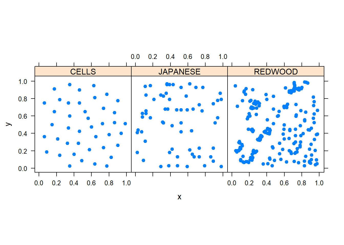
Here are three data examples including the spatial distribution of cell centres (left), California redwood trees (right), and Japanese black pine (middle). All data sets have been re-scaled to fit in to a one-by-one square.
5.1.1 \(G\) function: Nearest neighbour distances
For \(n\) events in a region \(A\), let \(y_i\) denote the distance from the \(i\)th event to the nearest other event in \(A\). Specifically, \[y_i = \min_{j\neq i} d({\mathbf{s}}_i,{\mathbf{s}}_j), i = 1,...,n,\] where \(d(\cdot,\cdot)\) is the distance function. The \(y_1, ..., y_n\) are called nearest neighbour distances. Define a random variable \(Y\) denoting the nearest neighbor distance with distribution \(G(y)={\mathbb{P}}(Y\leq y)\). \(y_1,...,y_n\) can be considered as a sample of \(Y\), and hence \(G(y)\) can be estimated by the following empirical distribution function (EDF), \[\hat G(y) = n^{-1} \#(y_i \leq y) = n^{-1}\sum_{i=1}^n \mathbf{1}_{\{y_i \leq y\}}.\] Under CSR, the actual \(G(y)\) depends on \(n\) and the region \(A\) and is not expressible in closed form because of edge effect. However, we can get an approximation of \(G(y)\) by ignoring the edge effects. Let \(|A|\) be the area of \(A\). Under CSR, given a specified event (\({\mathbf{s}}\)), the probability of an arbitrary event occurs within distance \(y\) of \({\mathbf{s}}\) is \(\pi y^2|A|^{-1}\), that is \[{\mathbb{P}}(\text{there exists an event } {\mathbf{s}}', \text{ such that } d({\mathbf{s}}', {\mathbf{s}}) \leq y) = \pi y^2|A|^{-1}.\] Since \(G(y)\) is the nearest distance among \(n-1\) distances, by the theory of distribution of order statistics, we conclude that \[G(y) = 1- (1-\pi y^2 |A|^{-1})^{n-1}.\] If \(n\) is large enough, a further approximation of \(G(y)\) is \[G(y) = 1- e^{-\lambda \pi y^2}, \ \text{where}\ \lambda = n|A|^{-1}.\] So if the point pattern data is under CSR, the EDF \(\hat G(y)\) should be close to the theoretical approximation of \(G(y)\). A plot of \(\hat G(y)\) versus theoretical approximation of \(G(y)\) would be a good exploratory tool to test the complete spatial randomness (CSR). If the nearest neighbor distances are shorter than expected, it suggests clustering/attraction; if the nearest neighbor distances are longer than expected, it suggests inhibition/regularity.
To formally test the complete spatial randomness (CSR), we can apply Monte Carlo test. Specifically, under CSR, the locations where the \(n\) events occur are independent and uniformly distributed in \(A\). So we can run \(m\) independent simulations, each of which generates \(n\) locations, say \(s_1^{(k)},..,s_n^{(k)}, k = 1,...,m\). For each simulation, we further calculated the nearest neighbor distances \(y_1^{(k)},...,y_n^{(k)}\) and eventually get the empirical distribution function \(\hat G^{(k)}(y)\). Define the upper simulation envelope \(U(y)\) and lower simulation envelope \(L(y)\) respectively as follows \[U(y) = \max_k \hat G^{(k)}(y),\ L(y) = \min_k \hat G^{(k)}(y).\] If the point pattern data is under CSR, the EDF of \(Y\) generated by original data should be between \(L(y)\) and \(U(y)\) with high probability.
Let \(\hat G^{(0)}(y)= \hat G(y)\). To be more precise, we use the following statistics \[u_k = \int \{\hat G^{(k)}(y)- \bar G(y)\}^2 dy, \ \text{where}\ \bar G(y) = m^{-1}\sum_{i=1}^m \hat G^{(i)}(y), k = 0,...,m.\] If the point pattern data is under CSR, \(u_0\) should not be in the right tail of ordered sequence of \(u_0, ..., u_m\). The empirical p value is \[(m+1)^{-1} \#(u_i \geq u_0) = (m+1)^{-1}\sum_{i=0}^m \mathbf{1}_{u_i \geq u_0}.\]
Now we apply the above methods to the three data examples, that are cell centres, California redwood trees, and Japanese black pine. First, we check the CSR for Japanese black pine data.
#CSR for Japanese black pines
library(splancs)
# computing and plotting nearest neighbour distances
npts<-65
japanese<-matrix(scan("./data//PPdata/japanese.txt"),npts,2,T)
par(pty="s")
poly<-matrix(c(0,0,1,0,1,1,0,1),4,2,T)
d<-nndistG(japanese)$dists
range(d)
## [1] 0.0100000 0.1204159dgrid<-0.001*(0:121)
ngrid<-length(dgrid)
Ghat<-rep(0,ngrid)
for (i in 1:ngrid) Ghat[i]<-sum(d<=dgrid[i])/npts
G0<-1-exp(-npts*pi*dgrid*dgrid)
plot(G0,Ghat,type="l", main = "JAPANESE")
#
# simulation envelope for complete spatial randomness
#
nsim<-99
Gmat<-matrix(0,ngrid,1+nsim); Gmat[,1]<-Ghat
set.seed(90123)
for (isim in 1:nsim) {
xy<-csr(poly,npts)
di<-nndistG(xy)$dists
for (i in 1:ngrid) Gmat[i,1+isim]<-sum(di<=dgrid[i])/npts
}
Gmax<-apply(Gmat[,2:(1+nsim)],1,max); Gmin<-apply(Gmat[,2:(1+nsim)],1,min)
lines(G0,Gmin,lty=2); lines(G0,Gmax,lty=2)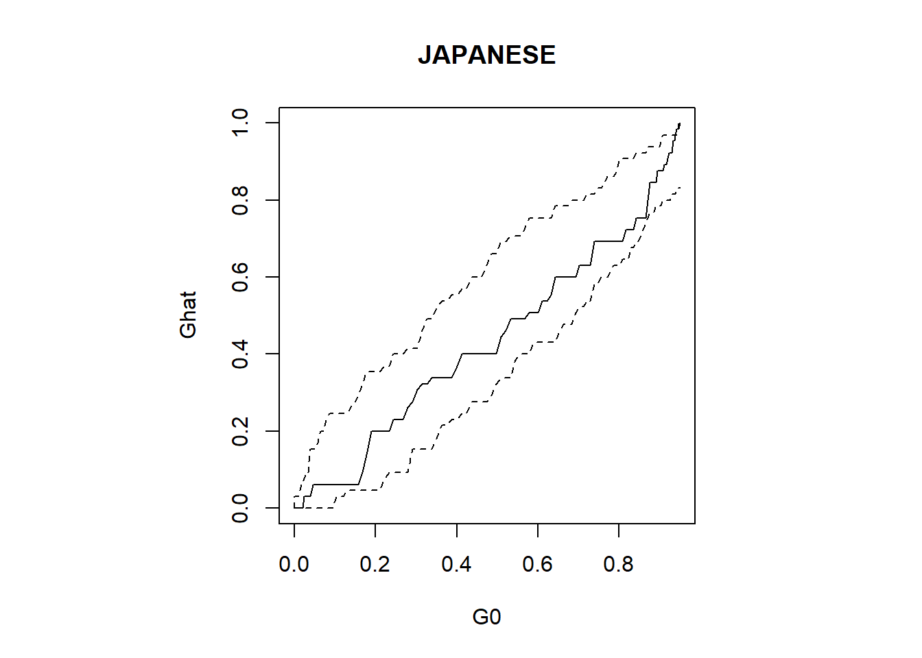
# Monte Carlo test
Gbar<-apply(Gmat,1,mean)
T<-sum((Ghat-Gbar)^2)
for (isim in 1:nsim) {
  T<-c(T,sum((Gmat[,1+isim]-Gbar)^2))
}
pval<-sum(T>=T[1])/(1+nsim)
pval
## [1] 0.65Similarly, we can apply the above codes for cell centres and California redwood trees data.
#CSR for redwood
npts<-62
redwood<-matrix(scan("./data//PPdata/redwood.txt"),npts,2,T)
par(pty="s")
poly<-matrix(c(0,0,1,0,1,1,0,1),4,2,T)
d<-nndistG(redwood)$dists
range(d)
## [1] 0.016 0.118dgrid<-0.001*(0:121)
ngrid<-length(dgrid)
Ghat<-rep(0,ngrid)
for (i in 1:ngrid) Ghat[i]<-sum(d<=dgrid[i])/npts
G0<-1-exp(-npts*pi*dgrid*dgrid)
plot(G0,Ghat,type="l", main = "redwood")
#
# simulation envelope for complete spatial randomness
#
nsim<-99
Gmat<-matrix(0,ngrid,1+nsim); Gmat[,1]<-Ghat
set.seed(90123)
for (isim in 1:nsim) {
xy<-csr(poly,npts)
di<-nndistG(xy)$dists
for (i in 1:ngrid) Gmat[i,1+isim]<-sum(di<=dgrid[i])/npts
}
Gmax<-apply(Gmat[,2:(1+nsim)],1,max); Gmin<-apply(Gmat[,2:(1+nsim)],1,min)
lines(G0,Gmin,lty=2); lines(G0,Gmax,lty=2)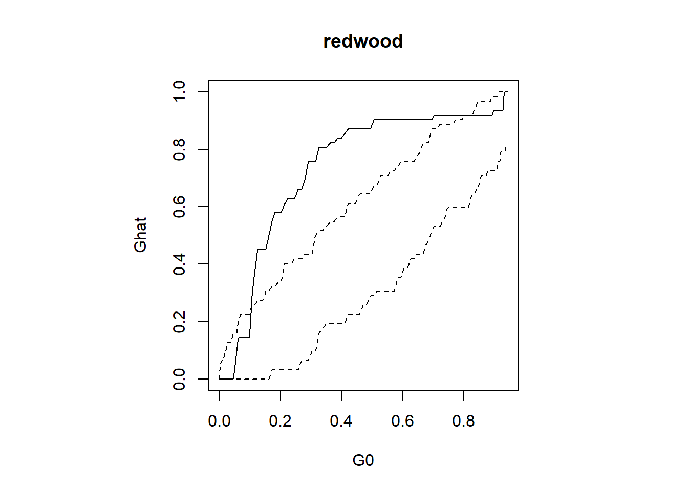
# Monte Carlo test
Gbar<-apply(Gmat,1,mean)
T<-sum((Ghat-Gbar)^2)
for (isim in 1:nsim) {
  T<-c(T,sum((Gmat[,1+isim]-Gbar)^2))
}
pval<-sum(T>=T[1])/(1+nsim)
pval
## [1] 0.01#CSR for cells
npts<-42
cells<-matrix(scan("./data/PPdata/cells.txt"),npts,2,T)
par(pty="s")
poly<-matrix(c(0,0,1,0,1,1,0,1),4,2,T)
d<-nndistG(cells)$dists
range(d)## [1] 0.08363014 0.15449595dgrid<-0.001*(0:155)
ngrid<-length(dgrid)
Ghat<-rep(0,ngrid)
for (i in 1:ngrid) Ghat[i]<-sum(d<=dgrid[i])/npts
G0<-1-exp(-npts*pi*dgrid*dgrid)
plot(G0,Ghat,type="l", main = "cells")
#
# simulation envelope for complete spatial randomness
#
nsim<-99
Gmat<-matrix(0,ngrid,1+nsim); Gmat[,1]<-Ghat
set.seed(90123)
for (isim in 1:nsim) {
xy<-csr(poly,npts)
di<-nndistG(xy)$dists
for (i in 1:ngrid) Gmat[i,1+isim]<-sum(di<=dgrid[i])/npts
}
Gmax<-apply(Gmat[,2:(1+nsim)],1,max); Gmin<-apply(Gmat[,2:(1+nsim)],1,min)
lines(G0,Gmin,lty=2); lines(G0,Gmax,lty=2)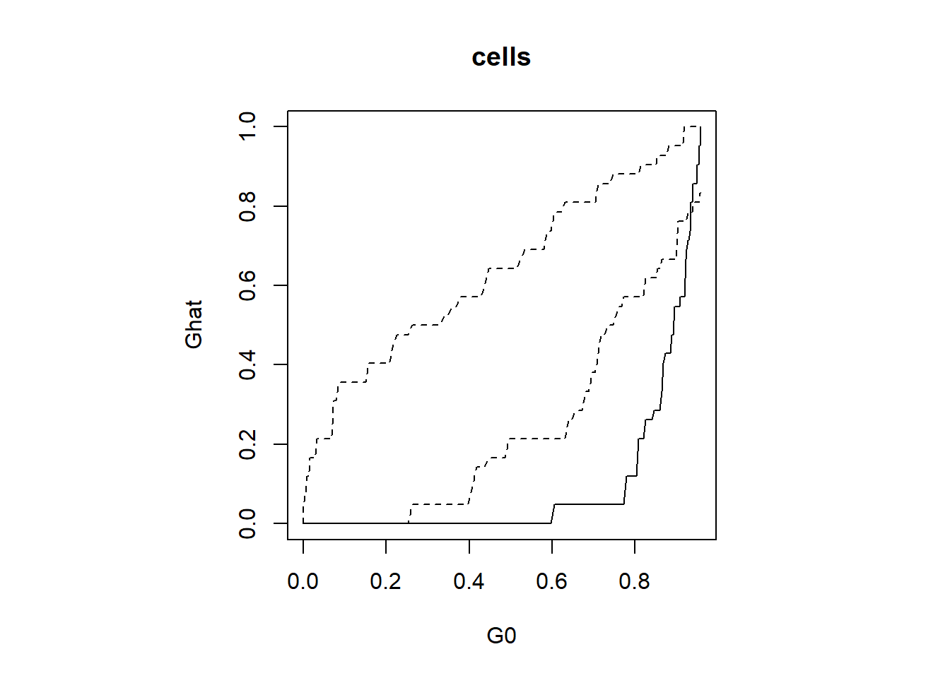
# Monte Carlo test
Gbar<-apply(Gmat,1,mean)
T<-sum((Ghat-Gbar)^2)
for (isim in 1:nsim) {
  T<-c(T,sum((Gmat[,1+isim]-Gbar)^2))
}
pval<-sum(T>=T[1])/(1+nsim)
pval
## [1] 0.015.1.2 \(F\) function: Point to nearest event distances
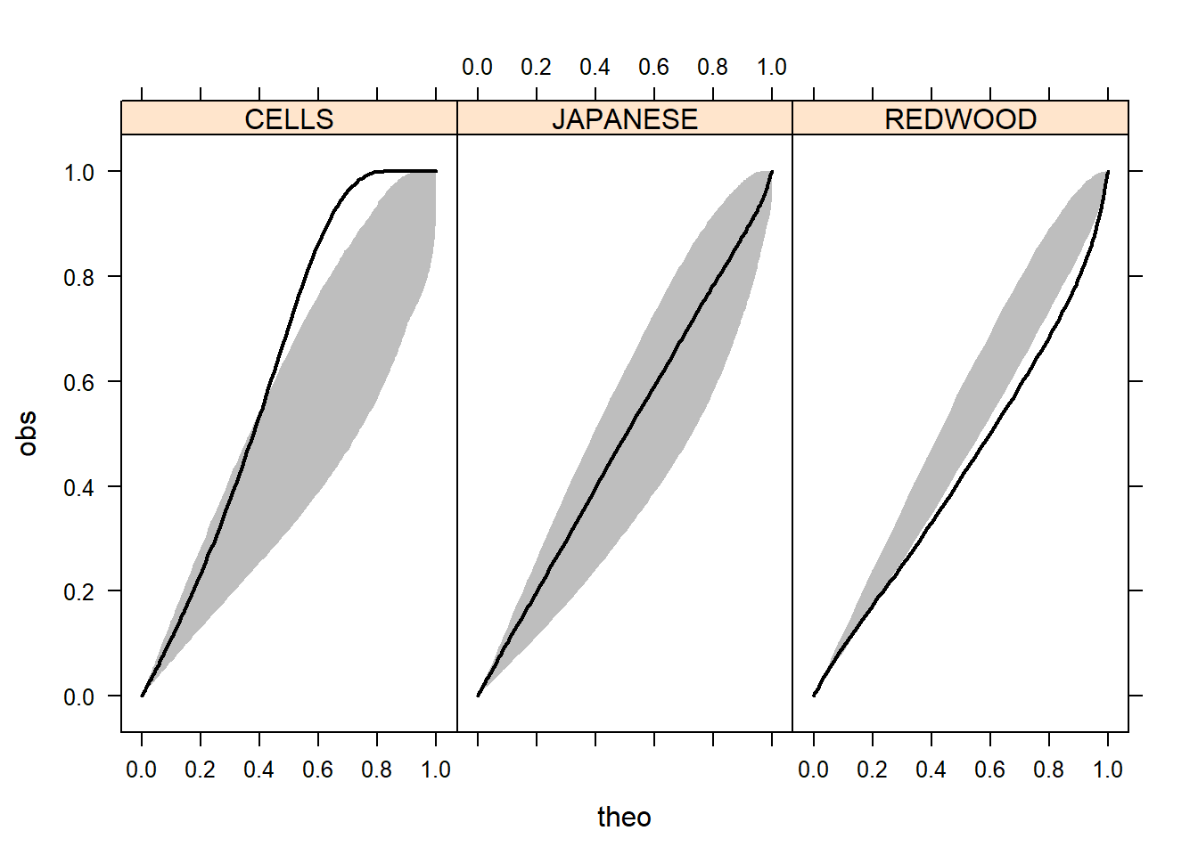
The F function measures the distribution of all distances from an arbitrary point of the plane to its nearest event. Assume \(n\) events occur in a region \(A\), say \({\mathbf{s}}_1,...{\mathbf{s}}_n\). We randomly sample \(m\) points in \(A\), say \(\tilde {\mathbf{s}}_1, ..., \tilde {\mathbf{s}}_m\). Let \(x_i\) denote the distance from \(\tilde {\mathbf{s}}_i\) to the nearest of the \(n\) events \({\mathbf{s}}_1,...,{\mathbf{s}}_n\). Specifically, \[x_i = \min_{1\leq j\leq n} d(\tilde {\mathbf{s}}_i,{\mathbf{s}}_j), i = 1,...,m.\] The \(x_1, ..., x_m\) are called point to nearest event distances. Define a random variable \(X\) denoting possible distance from an arbitrary point of the plane to its nearest event with distribution \(F(x)={\mathbb{P}}(X\leq x)\). This function is often called empty space function since it is a measure of the average space left between events. Specifically, \(1-F(x)\) measures the area of the region \(B(x)\) given by \[B(x) = \{{\mathbf{s}}:\min_{1\leq j\leq n} d({\mathbf{s}},{\mathbf{s}}_j) \geq x\}.\]
\(x_1,...,x_m\) can be considered as a sample of \(X\), and hence \(F(x)\) can be estimated by the following empirical distribution function (EDF), \[\hat F(x) = m^{-1} \#(x_i \leq x) = m^{-1}\sum_{i=1}^m \mathbf{1}_{\{x_i \leq x\}}.\]
By analogy with the procedure for nearest neighbour distances, under CSR, \(F(x)\) can be approximated by \[F(x) = 1- e^{-\lambda \pi x^2}, \ \text{where}\ \lambda = n|A|^{-1}.\] So if the point pattern data is under CSR, the EDF \(\hat F(x)\) should be close to the theoretical approximation of \(F(x)\). A plot of \(\hat F(x)\) versus theoretical approximation of \(F(x)\) would be a good exploratory tool to test the complete spatial randomness (CSR). If point to nearest event distances are longer than expected, it suggests clustering/attraction; if point to nearest events distances are shorter than expected, it suggests inhibition/regularity.
Further, a Monte Carlo test can be applied to testing of CSR based on the statistic \[u_k = \int \{\hat F^{(k)}(x)- \bar F(y)\}^2 dy, \ \text{where}\ \bar F(y) = \ell^{-1}\sum_{i=1}^\ell \hat F^{(i)}(x), k = 0,...,\ell,\] where \(\hat F^{(0)}(x)= \hat F(x)\).
Now we apply \(F\) function to the three data examples, that are cell centres, California redwood trees, and Japanese black pine.
rm(list=ls())
library(spatstat)
#Japanese black pine saplings example, measured in a square sampling region in a natural forest
data(japanesepines)
library(maptools)
spjpines <- as(japanesepines, "SpatialPoints")
spjpines1 <- elide(spjpines, scale=TRUE, unitsq=TRUE)
data(redwoodfull)
spred <- as(redwoodfull, "SpatialPoints")
data(cells)
spcells <- as(cells, "SpatialPoints")
r <- seq(0, sqrt(2), by = 0.001)
Fenvjap<-envelope(as(spjpines1, "ppp"), fun=Fest, r=r, nrank=1, nsim=99, verbose = FALSE)
#"nrank": the rank of the envelop in the simulated hat F();
#A rank of 1 means we take maximum and minimum as envelopes
Fenvred<-envelope(as(spred, "ppp"), fun=Fest, r=r, nrank=1, nsim=99, verbose = FALSE)
Fenvcells<-envelope(as(spcells, "ppp"), fun=Fest, r=r, nrank=1, nsim=99, verbose = FALSE)

#Merge results in a data frame
Fresults<-rbind(Fenvjap, Fenvred, Fenvcells)
Fresults<-cbind(Fresults, DATASET=rep(c("JAPANESE", "REDWOOD", "CELLS"), each=length(r)))
names(Fresults) <- c("r", "obs", "theo", "lo", "hi", "DATASET")

library(lattice)
print(xyplot(obs~theo|DATASET , data=Fresults, type="l",
             panel=function(x, y, subscripts)
             {
               lpolygon(c(x, rev(x)),
                        c(Fresults$lo[subscripts], rev(Fresults$hi[subscripts])),
                        border= FALSE, fill=TRUE, col = "gray")
               llines(x, y, col="black", lwd=2)
             }
))
5.1.3 Quadrant counts
An alternative method to a distance-based approach is to partition \(A\) into \(m\) subregions or quadrants, of equal area and to use the counts of numbers of events in the \(m\) quadrants to test CSR. For simplicity, assume that \(A\) is the unit square and is partitioned into a regular \(k\times k\) grids, so that \(m = k^2\). Let \(n_i, i=1,...,m\) be the quadrant counts and let \(\bar n = n/m\) be the sample mean of \(n_i\). Then a Pearson \(\chi^2\) test can be applied to testing CSR based on the statistic \[\chi^2 = \sum_{i=1}^m (n_i - \bar n)^2/\bar n.\] Under CSR, the statistic \(\chi^2\) approximately follows \(\chi^2\) distribution with degrees of freedom \(m-1\). A good approximation requires \(\bar n\) not too small. A conservative rule is \(\bar n\geq 5\).
5.2 Spatial point process
In this section, we introduce how to describe the point pattern data with a spatial point process. A spatial point process is a stochastic process each of whose realizations consists of a finite or countably infinite set of points in the plane. It is a stochastic process in which we observe the locations of some events of interest within a region \(A\).
Consider a spatial point process \({\mathbf{S}}\) in the domain \({\mathcal{D}}\subset {\mathbb{R}}^2\). Let \(N(A)\) be the number of events in an arbitrary region \(A\subset {\mathcal{D}}\). Then the distribution of a spatial point process is determined by its finite dimensional distribution (f.d.d.), specifically, for regions \(A_1,...A_n\), the f.d.d. of \({\mathbf{S}}\) is the distribution of the random vector \((N(A_1), ..., N(A_n))^\top\). The process \({\mathbf{S}}\) is stationary if the f.d.d. is invariant under translation and it is isotropic if it is invariant under translation and rotation.
Next, we’ll study the properties of the spatial point process \({\mathbf{S}}\) using the count process \(N(A)\) for any arbitrary \(A\subset {\mathcal{D}}\).
Let \(d{\mathbf{s}}\) be an infinitesimal region that contains the point \({\mathbf{s}}\). The first order property of the process \({\mathbf{S}}\) is described by its intensity function, which is defined by \[\lambda({\mathbf{s}}) = \lim_{|d{\mathbf{s}}| \rightarrow 0 } \frac{{\mathbb{E}}(N(d{\mathbf{s}}))}{|d{\mathbf{s}}|}.\] \(\lambda({\mathbf{s}})\) means the expected number of events per unit area centered at location \({\mathbf{s}}\). If \({\mathbf{S}}\) is stationary, \(\lambda({\mathbf{s}}) \equiv \lambda\), where \(\lambda\) is a constant.
For the second-order properties, we need to consider the set \({\mathbb{E}}[N(A_1)N(A_2)]\) with arbitrary \(A_1,A_2\subset D\) as a measure. The second-order intensity function is defined as \[ \lambda_2({\mathbf{s}}_1, {\mathbf{s}}_2) = \lim_{|d{\mathbf{s}}_1|, |d{\mathbf{s}}_2| \rightarrow 0} \frac{{\mathbb{E}}[N(d{\mathbf{s}}_1)N(d{\mathbf{s}}_2)]}{|d{\mathbf{s}}_1||d{\mathbf{s}}_2|}.\] The reweighted second-order intensity (or genearl pair correlation function) is defined by scaling the \(\lambda_2({\mathbf{s}}_1,{\mathbf{s}}_2)\), \[\rho({\mathbf{s}}_1,{\mathbf{s}}_2) = \frac{\lambda_2({\mathbf{s}}_1,{\mathbf{s}}_2)}{\lambda({\mathbf{s}}_1)\lambda({\mathbf{s}}_2)}.\] Let \(h= {\mathbf{s}}_2-{\mathbf{s}}_1\) and \(r = ||{\mathbf{s}}_2 -{\mathbf{s}}_1||\). If the process \({\mathbf{S}}\) is stationary, \(\lambda_2({\mathbf{s}}_1,{\mathbf{s}}_2) = \lambda_2(h)\) and \(\rho({\mathbf{s}}_1,{\mathbf{s}}_2)= \lambda_2(h)/\lambda^2\). Further, if the process \({\mathbf{S}}\) is isotropic, \(\lambda_2({\mathbf{s}}_1,{\mathbf{s}}_2) = \lambda_2(r)\) and \(\rho({\mathbf{s}}_1,{\mathbf{s}}_2) = \lambda_2(r)/\lambda^2 \triangleq \rho(r)\). If the point pattern data is under complete spatial randomness (CSR), \(\rho({\mathbf{s}}_1,{\mathbf{s}}_2) = 1\).
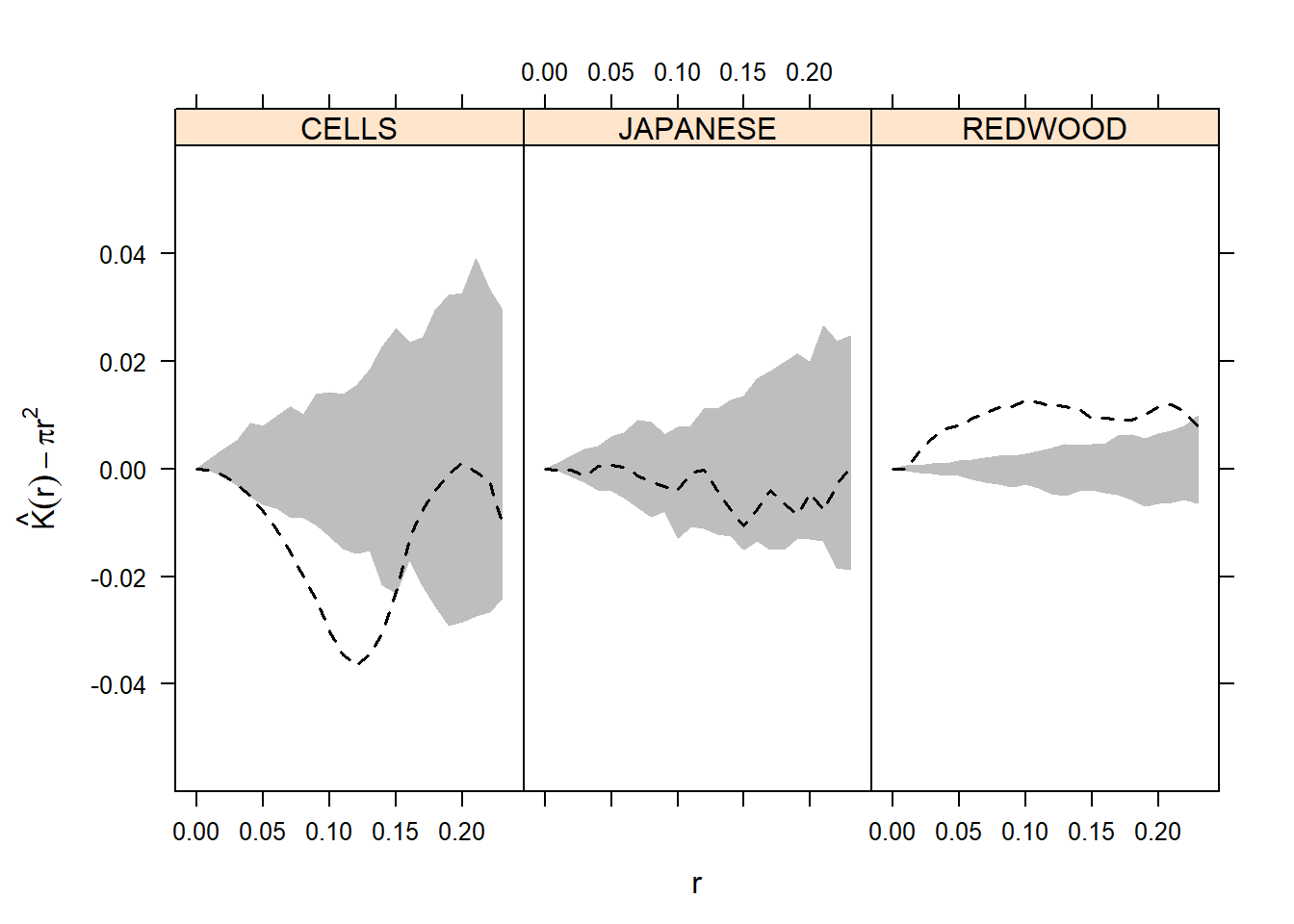
5.2.1 Ripley’s \(K\) function
The \(K\) function was introduced by Ripley (1977) and its estimator is widely used as descriptive statistic for stationary spatial point process. Rather than nearest neighbor distances, the \(K\) function considers the expected number of points within distance \(d\) of an arbitrary point, say \({\mathbf{s}}\), but not including the points \({\mathbf{s}}\). Under stationarity, this expectation is the same for any point. Specifically, let \(b_o({\mathbf{s}},r)\) be the disc centered at \({\mathbf{s}}\) with radius \(r\), but excluding the center point \({\mathbf{s}}\), \[ K(r) = {\mathbb{E}}(N(b_o({\mathbf{s}},r)))/\lambda.\] Under CSR, we can calculate it explicitly, \[K(r) = \lambda \pi r^2 /\lambda = \pi r^2,\] which is the area of the disc with radius \(r\). If the point pattern data were observed at \({\mathbf{s}}_1,...,{\mathbf{s}}_n\), a customary estimate of \(K(h)\) is \[\hat K(r) = \hat \lambda^{-1}n^{-1}\sum_{i=1}^n\sum_{j\neq i} \mathbf{1}_{\{||{\mathbf{s}}_i - {\mathbf{s}}_j|| \leq r\}}.\] However, \(\hat K(r)\) is negatively biased because of edge-effect. A way to fix this is we can add weights in the sums of \(\hat K(r)\). Let \(w({\mathbf{s}},r)\) be the proportion of the circumference of the circle with center \({\mathbf{s}}\) and radius \(r\) which lies within the domain of interest \({\mathcal{D}}\). Let \(w_{ij} = w({\mathbf{s}}_i, ||{\mathbf{s}}_i-{\mathbf{s}}_j||)\). Then, an unbiased estimator of \(K(r)\) is \[\hat K(r) = \hat \lambda^{-1}n^{-1}\sum_{i=1}^n\sum_{j\neq i} w_{ij}^{-1} \mathbf{1}_{\{||{\mathbf{s}}_i - {\mathbf{s}}_j|| \leq r\}}.\] The estimate of \(\lambda\) is \(\hat \lambda = n/|{\mathcal{D}}|\). Finally, we obtain the estimator of \(K(r)\) is \[\hat K(r) = n^{-2}|{\mathcal{D}}|\sum_{i=1}^n\sum_{j\neq i} w_{ij}^{-1}\mathbf{1}_{\{||{\mathbf{s}}_i - {\mathbf{s}}_j|| \leq r\}}.\]
Remarks:
i). We often check \(\hat K(r)\) for \(r\) small. Large \(r\) may lead to \(w_{ij}^{-1}\) very large. The sampling fluctuations in \(\hat K(r)\) increase with \(r\) as well.
ii). Regularity/inhibition of spatial point pattern data implies \(\hat K(r) < \pi r^2\); clustering implies \(\hat K(r) > \pi r^2\). A plot of \(L(r) = \hat K(r) - \pi r^2\) vs \(r\) has been proposed to check CSR. Evidently, \(L(r) = 0\) under CSR, suggesting we look for peaks and valleys in the plot. For instance, a peak at distance \(r_0\) would suggest clustering at that distance.
iii). If the point process is isotropic, we can connect \(K(r)\) to \(\rho(r)\), the pair correlation function. Here is the relationship, \[\rho(r) = \frac{K'(r)}{2\pi r}.\] A proof of the above formula:
Assume that \({\mathbb{E}}(N(d{\mathbf{s}})) \sim {\mathbb{P}}(N(d{\mathbf{s}}) = 1)\) in the sense that the ratio of these two quantities tends to \(1\) and \(|d{\mathbf{s}}| \to 0\) and further assume that \({\mathbb{E}}(N(d{\mathbf{s}})N(d\tilde {\mathbf{s}}))\sim {\mathbb{P}}(N(d{\mathbf{s}}) =1, N(d\tilde {\mathbf{s}}) = 1)\). Then \[{\mathbb{P}}(N(d\tilde {\mathbf{s}}) = 1 | N(d{\mathbf{s}}) = 1) \sim \lambda_2(\tilde {\mathbf{s}}, {\mathbf{s}})d\tilde {\mathbf{s}}/\lambda({\mathbf{s}}) = \lambda\rho(||\tilde {\mathbf{s}}-{\mathbf{s}}||) |d\tilde {\mathbf{s}}|,\] and hence \[\lambda K(r) = {\mathbb{E}}(N(b_o({\mathbf{s}},r))) = \int_{0}^r \lambda\rho(x) (2\pi xdx).\] Taking derivative with respect to \(r\), we get \(\rho(r) = \frac{K'(r)}{2\pi r}\).
Now we apply \(K\) function to the three data examples, that are cell centres, California redwood trees, and Japanese black pine.
rm(list=ls())
library(spatstat)
#Japanese black pine saplings example, measured in a square sampling region in a natural forest
data(japanesepines)
library(maptools)
spjpines <- as(japanesepines, "SpatialPoints")
spjpines1 <- elide(spjpines, scale=TRUE, unitsq=TRUE)
data(redwoodfull)
spred <- as(redwoodfull, "SpatialPoints")
data(cells)
spcells <- as(cells, "SpatialPoints")
r <- seq(0, sqrt(2)/6, by = 0.01)

Kenvjap<-envelope(as(spjpines1, "ppp"), fun=Kest, r=r, nrank=2, nsim=99, verbose = FALSE)
Kenvred<-envelope(as(spred, "ppp"), fun=Kest, r=r, nrank=2, nsim=99, verbose = FALSE)
Kenvcells<-envelope(as(spcells, "ppp"), fun=Kest, r=r, nrank=2, nsim=99, verbose = FALSE)

#Merge results in a data frame
Kresults<-rbind(Kenvjap, Kenvred, Kenvcells)
Kresults<-cbind(Kresults,
   DATASET=rep(c("JAPANESE", "REDWOOD", "CELLS"), each=length(r)))
names(Kresults) <- c("r", "obs", "theo", "lo", "hi", "DATASET")

library(lattice)
print(xyplot((obs-theo)~r|DATASET , data=Kresults, type="l",
             ylim= c(-.06, .06), ylab=expression(hat(K) (r)  - pi * r^2),
             panel=function(x, y, subscripts)
             {
               Ktheo<- Kresults$theo[subscripts]

               lpolygon(c(r, rev(r)),
                        c(Kresults$lo[subscripts]-Ktheo, rev(Kresults$hi[subscripts]-Ktheo)),
                        border="gray", fill=TRUE, col = "gray"
               )

               llines(r, Kresults$obs[subscripts]-Ktheo, lty=2, lwd=1.5, col="black")
             }
))
5.2.2 The homogeneous (planar) Poisson process
The underlying process for spatial point pattern data under complete spatial randomness (CSR) is called homogeneous planar Poisson process, which is the cornerstone on which the theory of spatial point process is built. Recall the definition of CSR. Now we use it to define homogeneous Poisson process on \({\mathbb{R}}^2\).
the number of events in any planar region \(A\subset {\mathbb{R}}^2\) with area \(|A|\) follows a Poisson distribution with mean \(\lambda |A|\);
given \(n\) events in a region \(A\), say \({\mathbf{s}}_1,...{\mathbf{s}}_n\), the \({\mathbf{s}}_i\)s are an independent random sample from the uniform distribution on \(A\). Here \({\mathbf{s}}_i\) denotes the coordinate where the \(i\)th event occurs.
Properties of homogeneous Poisson process on \({\mathbb{R}}^2\):
i). The intensity function is constant, \(\lambda\).
ii). The second order intensity function is constant, \(\lambda^2\).
iii). The \(K\) function is \(K(r) = \pi r^2\).
iv). The variance of number of events occur at region \(A\) is \(\text{Var}(N(A)) = \lambda |A|.\)
v). The \(F\) function and \(G\) functions are identical and can be derived by \[F(x) = G(x) = P(N(b_o({\mathbf{s}},x) > 0) = 1 - \exp(-\lambda \pi x^2), x> 0.\]
5.3 Models
In this section, we’ll introduce some simple construction for spatial point process to describe clustering or regularity of point pattern data.
5.3.1 Poisson cluster processes
Neyman and Scott (1958) introduced Poisson cluster processes, which were used to model aggregated spatial point patterns. Here is the definition.
Parent events from a Poisson process with intensity \(\rho\).
Each parent produces a random number \({\mathbf{N}}\) of offspring, realized independently and identically for each parent according to a probability distribution \({\mathbb{P}}({\mathbf{N}}= k) = p_k, k=0,1,...\).
The positions of the offspring relative to their parents are independently and identically distributed according to a bivariate pdf \(h(\cdot)\). For example, \(h\) can be a radially symmetric Gaussian distribution, that is \[h(s_x,s_y) = (2\pi\sigma^2)^{-1}e^{-\frac{s_x^2+s_y^2}{2\sigma^2}}.\] Conventionally, the final pattern consists of the offspring only.
Properties of Poisson cluster processes:
i). Stationary with intensity \(\lambda = \rho \mu\) where \(\mu = {\mathbb{E}}({\mathbf{N}})\). Isotropic if \(h\) is radially symmetric.
ii). \(K\) function is \[K(r) = \pi r^2 + {\mathbb{E}}({\mathbf{N}}({\mathbf{N}}-1))H_2(r)/(\rho \mu^2),\] where \(H_2(r)\) is the cumulative distribution function (cdf) of the difference between the positions of two offspring from the same parent.
The pdf of the difference between the positions of two offspring from the same parent is given by \[h_2(\tilde {\mathbf{s}}) = \int h({\mathbf{s}})h({\mathbf{s}}-\tilde {\mathbf{s}})d{\mathbf{s}}.\]
Remarks:
a). As \(r \to \infty\), \(K(r) - \pi r^2 \to c:= {\mathbb{E}}({\mathbf{N}}({\mathbf{N}}-1))/(\rho \mu^2)\). If \({\mathbf{N}}\) follows Poisson distribution, \(c = \rho^{-1}\).
b). Derivation of \(K\) function: If we consider an arbitrary event \({\mathbf{s}}_1\) within a cluster size \({\mathbf{N}}\), the expected number of other events from the same cluster within a distance \(r\) is \[\sum_{i=2}^{\mathbf{N}}{\mathbb{E}}(\mathbf{1}_{d({\mathbf{s}}_i,{\mathbf{s}}_1)\leq r}) = ({\mathbf{N}}-1)H_2(r).\] Given an arbitrary event \({\mathbf{s}}_1\) belongs to the cluster with size \({\mathbf{N}}\), the probability distribution of \({\mathbf{N}}\) is obtained by length-biased sampling from \[{\mathbb{P}}({\mathbf{N}}= k | \text{an event is sighted in the cluster}) = kp_k/\mu, k = 1,2,....\] Then given an arbitrary event \({\mathbf{s}}_1\), the expected number of other events from the same cluster within a distance \(r\) of \({\mathbf{s}}_1\) is \[\sum_{k=1}^\infty (k-1)H_2(r)\times (kp_k)/\mu = {\mathbb{E}}({\mathbf{N}}({\mathbf{N}}-1))H_2(r)/\mu.\] On the other hand, the expected number of unrelated events, meaning events from different clusters, within distance \(r\) of an arbitrary event, is \(\lambda \pi r^2.\)
Therefore, \[\lambda K(r) = \lambda \pi r^2 + {\mathbb{E}}({\mathbf{N}}({\mathbf{N}}-1))H_2(r)/\mu.\]
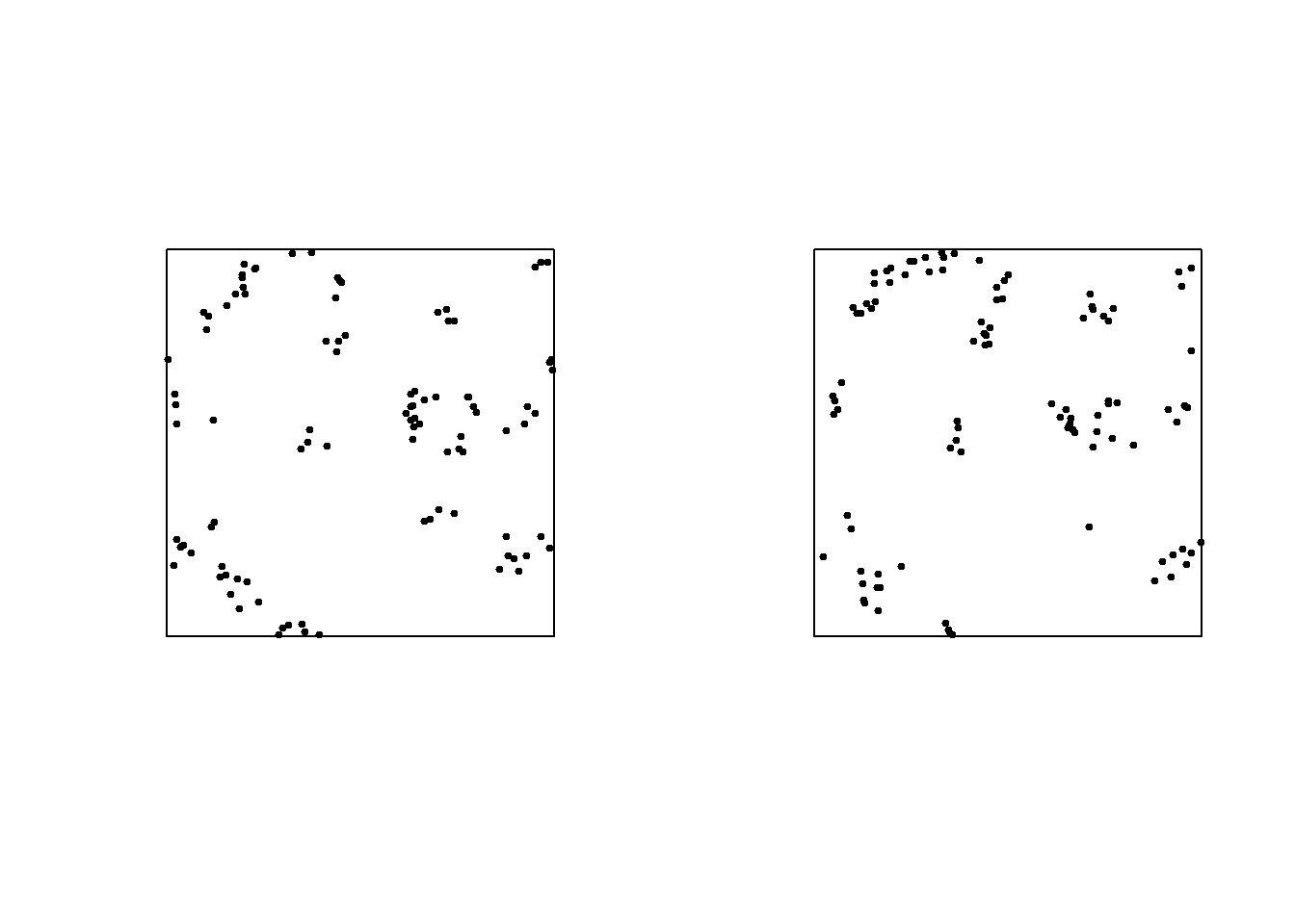
c). length-biased sampling: Suppose that the probability of an arbitrary event occurs at a small disc \(b({\mathbf{s}}, d{\mathbf{s}})\) is \(\theta:=\lambda |d{\mathbf{s}}|\), which is close to zero. Given the cluster size \({\mathbf{N}}= k\), the probability that the event is sighted at this specific cluster is \[{\mathbb{P}}(\text{the event is sighted at the cluster} | {\mathbf{N}}= k) = 1-(1-\theta)^k := w_k.\] Then \[{\mathbb{P}}({\mathbf{N}}= k|\text{the event is sighted at the cluster} ) = \frac{w_kp_k}{\sum_{k} w_kp_k}.\] Since \(w_k \approx k\theta\) when \(\theta \to 0\), we have \[{\mathbb{P}}({\mathbf{N}}= k|\text{the event is sighted at the cluster} ) \approx \frac{kp_k}{\sum_{k} kp_k}=kp_k/\mu.\] Here are two simulated Poisson cluster processes, each with 25 parents on the unique square an average of four offspring per parent and radially symmetric Gaussian dispersion of offspring, with parameter \(\sigma = 0.025\). In the left-hand panel, each parent has exactly four offspring. In the right-hand panel, offspring are randomly allocated amongst the 25 parents.
5.3.2 Inhomogeneous Poisson processes
The inhomogeneous Poisson processes are introduced to describe point process with spatially varying intensity function. Here is the definition.
(i). \(N(A)\) has a Poisson distribution with mean \(\int_A \lambda({\mathbf{s}})d{\mathbf{s}}.\)
(ii). Given \(N(A) = n\), the \(n\) events in \(A\) form an independent random sample from the distribution on \(A\) with pdf proportional to \(\lambda({\mathbf{s}})\).
The inhomogeneous Poisson process provides a possible framework for the introduction of covariates into the analysis of spatial point pattern via modeling \(\lambda({\mathbf{s}})\) as a function of potential predictors, say \(X_1({\mathbf{s}}),...,X_p({\mathbf{s}})\).
For example, suppose that the locations of trees of a particular species are thought to follow a Poisson process with intensity determined by height above sea-level, then a possible model might be
\[\lambda({\mathbf{s}}) = e^{\alpha + \beta X({\mathbf{s}})},\] where \(X({\mathbf{s}})\) denotes height above sea-level at the location \({\mathbf{s}}\). Cox (1972a) refers to this as a “modulated Poisson process”.
The figure below shows a partial realization of an inhomogeneous Poisson process with \(A\) the unit square, \(N(A)=100\) and \(\lambda({\mathbf{s}}) = e^{-2s_x-s_y}\). 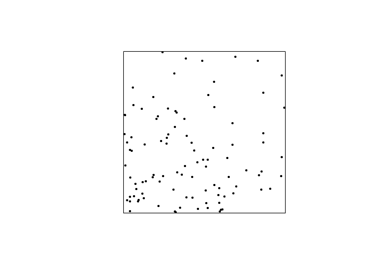
5.3.3 Cox process and Log-Gaussian Cox processes
The rationale behind the use of Poisson cluster processes as models for biological processes is that aggregated spatial point patterns might be generated by the clustering of groups of related events. A second possible source of aggregation is environmental heterogeneity. Specifically, an inhomogeneous Poisson process with intensity function \(\lambda({\mathbf{s}})\) will produce apparent clusters of events in regions of relatively high intensity. The source of such environmental heterogeneity might itself be stochastic in nature. This suggests investigation of a class of “doubly stochastic” processes formed as inhomogeneous Poisson processes with stochastic intensity functions. Such processes are called Cox processes, following their introduction in one temporal dimension by Cox (1955). Explicitly, a spatial Cox process can be defined by
\(\{\Lambda({\mathbf{s}}) : {\mathbf{s}}\in {\mathbb{R}}^2\}\) is a non-negative-valued stochastic process.
Given \(\Lambda({\mathbf{s}}) = \lambda({\mathbf{s}})\), the event form an inhomogeneous Poisson with intensity function \(\lambda({\mathbf{s}})\).
Remarks:
a). A Cox process is stationary if and only if its intensity process \(\Lambda({\mathbf{s}})\) is stationary, and similar for isotropy. In the stationary case, the intensity is \[\lambda = {\mathbb{E}}(\Lambda({\mathbf{s}})).\] Also, in the stationary and isotropic case, the second-order intensity function is \[\lambda_2({\mathbf{s}}, \tilde {\mathbf{s}}) = {\mathbb{E}}(\Lambda({\mathbf{s}})\Lambda(\tilde {\mathbf{s}})) = \lambda^2 + \text{Cov}(\Lambda({\mathbf{s}}), \Lambda(\tilde{\mathbf{s}})),\] and the pair correlation function is \[\rho(r) = 1+\text{Cov}(\Lambda({\mathbf{s}}), \Lambda(\tilde{\mathbf{s}}))/\lambda^2.\]
So if the random field \(\Lambda({\mathbf{s}})\) has positive autocorrelations, then the resulting point pattern is clustered.
The log-Gaussian Cox process is one of the most widely applicable Cox processes.
Log-Gaussian Cox process: Suppose that \(X({\mathbf{s}})\) is a stationary and isotropic Gaussian random field with mean \(\mu_X\) and variance \(\sigma_X^2\) and covariance function \(C_X(r)\). Define the intensity process \[\Lambda({\mathbf{s}}) = e^{X({\mathbf{s}})}.\] Then the intensity of the corresponding Cox process is \[\lambda = e^{\mu_X + \frac{1}{2}\sigma_X^2}.\] and the pair correlation function is \[\rho(r) = 1+{\mathbb{E}}(\Lambda({\mathbf{s}})\Lambda(\tilde {\mathbf{s}}))/\lambda^2 = e^{C_X(r)}.\]
5.3.4 Hard-core point processes
A hard-core point process is a point process in which there are no points at a distance smaller than a specific minimum distance denoted by \(r_0\). Hard-core processes are typical examples of processes with a tendency towards regularity, which results from repulsion among the points.
There are two main types of hard-core processes:
1). Processes resulting from thinning operations. These operations may remove points that are close to other points or eliminate points in clusters to producing a pattern of isolated points. Consider, for example, ecological processes in plant communities, where dense patterns of seedlings develop into hard-core patterns as a result of competition. Different thinning rules generate different patterns and models.
2). Processes resulting from interaction of hard objects. Here the objects represented by the pattern are hard and non-penetrable such that if they are randomly distributed in space they cannot be closer together than permitted by their sizes. These objects can exist either simultaneously from the very beginning or can appear over time.
5.4 Model fitting
5.4.1 Parameter estimation using the \(K\)-function
In this section, we describe a method of parameter estimation using \(K(r)\) and its estimator \(\hat K(r)\). Suppose that our model incorporates a vector of parameters \({\boldsymbol{\theta}}\). Let \(K(r;{\boldsymbol{\theta}})\) denote the theoretical \(K\)-function and \(\hat K(r)\) the estimator derived in section 5.2.1, which is \[\hat K(r) = \hat \lambda^{-1}n^{-1}\sum_{i=1}^n\sum_{j\neq i} w_{ij}^{-1} \mathbf{1}_{\{||{\mathbf{s}}_i - {\mathbf{s}}_j|| \leq r\}}.\] A “least square” idea to measure the discrepancy between model and data is given by
\[D({\boldsymbol{\theta}}) = \int_0^{t_0} w(t)[\hat K^c(t) - K^c(t;{\boldsymbol{\theta}})]^2 dt,\] where the constant \(t_0\) and \(c\), and the weighting function \(w(t)\) are to be chosen. We then estimate \({\boldsymbol{\theta}}\) by minimizing \(D({\boldsymbol{\theta}})\).
In practice, we can pick \(w(t) = 1\), \(c = 0.5 \ \text{or}\ 0.25\) (to stabilize the variability of \(\hat K(r)\)), and not too large \(t_0\), for example, \(t_0 = 0.25 \min(a,b)\) for data on a rectangular region with side-length \(a\) and \(b\).
Now we simulate a Poisson cluster processes with \(\rho = 25\), \(\mu = 40\), and radially symmetric Gaussian distribution \(h\), that is \[h(s_x,s_y) = (2\pi\sigma^2)^{-1}e^{-\frac{s_x^2+s_y^2}{2\sigma^2}},\] where \(\sigma^2\) is set to \(0.05\). We applied the above methods with the simulated data to obtaining an estimate of \(\rho\) and \(\sigma^2\).
To obtain the explicit formula of \(K(t;{\boldsymbol{\theta}})\), we need to find \(H_2(r)\) first. When \(h\) is a radially symmetric Gaussian distribution, \(H_2(r)\) has explicit form.
Assume the coordinate of a parent is \({\mathbf{s}}=(s_x,{\mathbf{s}}_y)\), and two of its children located at \({\mathbf{s}}_1\) and \({\mathbf{s}}_2\), which are random. When \(h\) is Gaussian, \[{\mathbf{s}}_1 \sim \text{Gaussian}({\mathbf{s}}, \sigma^2),\ {\mathbf{s}}_2 \sim \text{Gaussian}({\mathbf{s}}, \sigma^2).\] Let \(\Delta\) be the difference of \({\mathbf{s}}_1\) and \({\mathbf{s}}_2\) whose distribution is \(H_2(\Delta_x,\Delta_y)\). Since \({\mathbf{s}}_1\) and \({\mathbf{s}}_2\) are independent, the distribution of \(\Delta\) is \[\Delta\sim \ \text{Gaussian}(\mathbf{0}, 2\sigma^2).\] Therefore, given \(r\), \[H_2(r) = {\mathbb{P}}(\Delta_x^2 + \Delta_y^2 \leq r^2) = \int_0^r \int_0^{2\pi} \frac{1}{4\pi\sigma^2}e^{-\frac{t^2}{4\sigma^2}}td\theta dt= 1- e^{-\frac{r^2}{4\sigma^2}}.\]
Now we are ready to implement the simulation and estimation procedures in R.
rm(list=ls())
#fitting using the K-function

#simulate a Poisson cluster process.
library(splancs)
PCP<-function(n,rho,sigma,a=1,b=1,poisson=TRUE) {
  #
  # Simulation of Poisson cluster process on rectangle (0,a)X(0,b),
  # with toroidal wrapping
  #
  # Arguments
  #
  #          n: number of events
  #        rho: mean number of parents per unit area
  #     sigma: standard deviation of Gaussian dispersion of offspring relative
  #            to their parents in either coordinate direction
  #      a, b: dimensions of rectangle
  #   poisson: if TRUE, offspring are randomly distributed amongst parents,
  #            if false the number of offspring per parent is constant (with
  #            adjustment to n if n/(rho*a*b) is non-integer)
  #
  # Result
  #
  #   A two-column matrix of event locations (x,y)
  #
  m<-round(rho*a*b)
  if (poisson==FALSE) {
    k<-round(n/m)
    n<-m*k
  }
  xp<-a*runif(m)
  yp<-b*runif(m)
  if (poisson==FALSE) parent<-rep(1:m,k) else parent<-sample(1:m,n,replace=TRUE)
  xoff<-xp[parent]+sigma*rnorm(n)
  yoff<-yp[parent]+sigma*rnorm(n)
  take<-(xoff>a)
  if (sum(take)>0) {
    xoff[take]<-xoff[take]-a*floor(xoff[take]/a)
  }
  take<-(yoff>b)
  if (sum(take)>0) {
    yoff[take]<-yoff[take]-b*floor(yoff[take]/b)
  }
  take<-(xoff<0)
  if (sum(take)>0) {
    xoff[take]<-a+xoff[take]+a*ceiling(xoff[take]/a)
  }
  take<-(yoff<0)
  if (sum(take)>0) {
    yoff[take]<-b+yoff[take]+b*ceiling(yoff[take]/b)
  }
  cbind(xoff,yoff)
}

# Poisson cluster processes;
# the number of offspring follows Poisson(4)
set.seed(1351)
xy<-PCP(1000,25,0.05,poisson=FALSE)
par(pty="s",mfrow=c(1,2))
pointmap(xy,pch=19,cex=0.5,xaxt="n",yaxt="n",bty="n",xlim=c(0,1),ylim=c(0,1))
square<-matrix(c(0,0,1,0,1,1,0,1),4,2,byrow=TRUE)
polymap(square,add=TRUE)
#

#estimated K function.
library(spatstat)
X <- as.ppp(xy, c(0,1,0,1))
K.est <- Kest(X, correction = "Ripley")
plot(K.est)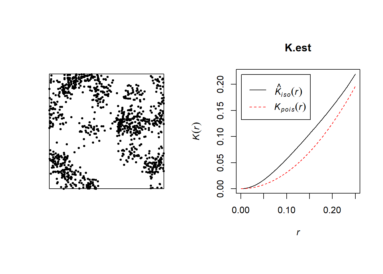
r.v <- K.est$r
K.v <- K.est$iso
n <- length(r.v)

#theoretical K function
theo.K <- function(rho, sigma, r) {
  tmp <- pi * r^2 + 1/rho*(1-exp(-r^2/4/sigma^2))
  return(tmp)
}


#c
c <- 0.25


#cost function
d.theta <- function(par, c0 = c, n0 = n, r = r.v, K = K.v) {
  rho <- par[1]
  sigma <- par[2]
  theoK.v <- sapply(1:n0, function(m) theo.K(rho, sigma, r[m]))
  di <- sum(sapply(1:n0, function(m) (theoK.v[m]^c0 - K[m]^c0)^2))
  return(di)
}

init <- c(10,1)

options("scipen"=100, "digits"=4)
optim(init, d.theta, method = "L-BFGS-B", lower = c(0.1, 0.0001), upper = c(100, 10))
## $par
## [1] 29.36854 0.04357
##
## $value
## [1] 0.004901
##
## $counts
## function gradient
## 37 37
##
## $convergence
## [1] 0
##
## $message
## [1] "CONVERGENCE: REL_REDUCTION_OF_F <= FACTR*EPSMCH"In this estimation procedure, \(\rho\) and \(\sigma^2\) cannot be estimated well, but \(\rho \sigma^2\) is estimated well. In the above example, \(\rho \sigma^2 = 25\times 0.05 = 1.25\) and \(\hat \rho \hat \sigma^2 = 29.37854\times 0.04357 = 1.28\). Indeed, we can check the behavior of \(K(r)\) around \(r=0\) by Taylor’s expansion, \[K(r) \approx \pi r^2 + r^2/(4\rho \sigma^2),\] from where we can see \(\rho\) and \(\sigma^2\) are not separately identifiable.
5.4.2 Likelihood inference for inhomogeneous Poisson processes
Consider an inhomogeneous Poisson process with intensity function \(\lambda({\mathbf{s}})\) in a region \(A\). Suppose that we observe \(n\) events at \({\mathbf{S}}= \{{\mathbf{s}}_1,...,{\mathbf{s}}_n\}\). The likelihood for \(\lambda(\cdot)\) given the data \({\mathbf{S}}\) can be factorized as the product of the probability that the number of events is \(n\) and the probability that the events are located at \({\mathbf{S}}\). Specifically, \[\frac{\lambda_A^n}{n!} e^{-\lambda_A}\times\prod_{i=1}^n \frac{\lambda({\mathbf{s}}_i)}{\lambda_A}, \] where \[\lambda_A = \int_A \lambda({\mathbf{s}}) d{\mathbf{s}}.\] So the log-likelihood for \(\lambda(\cdot)\) is \[\sum_{i=1}^n \log \lambda({\mathbf{s}}_i) - \lambda_A - \log(n!).\] Ignoring the constant \(\log(n!)\), we get \[L(\lambda) = \sum_{i=1}^n \log \lambda({\mathbf{s}}_i) - \lambda_A.\] If we model the log transformation of \(\lambda({\mathbf{s}})\) with a regression model with covariates \(X_1({\mathbf{s}}),...,X_p({\mathbf{s}})\), that is \[\log(\lambda({\mathbf{s}})) = \sum_{j=1}^p \beta_j X_j({\mathbf{s}}),\]
then the log-likelihood is
\[L({\boldsymbol{\beta}}) = \sum_{i=1}^n \sum_{j=1}^p \beta_j X_j({\mathbf{s}}_i) - \int_A e^{\sum_{j=1}^p \beta_j X_j({\mathbf{s}})}d{\mathbf{s}}.\]
To maximizing the log-likelihood, we need to evaluate the integration in \(L({\boldsymbol{\beta}})\), where we need know the values of predictors \(X_j\) in any location in \(A\). If we just use spatial coordinates \(s_x,s_y\) as predictors, it is fine. However, most of time \(X_j\)s only are discrete observations. In such case, we may need model \(X_j\)s and do interpolations to get values of \(X_j\)s in other locations.
Now we use the Lansing Woods data to illustrate the above method. The Lansing Woods data provide locations of 2251 trees, including three major species groupings of hickories, maples and oaks in a 19.6 acre square plot in Lansing Woods, Clinton County, Michigan.
rm(list=ls())
#likelihood fitting for inhomogeneous Poisson process
library(cubature)
data(lansing)
x <- as.points(lansing[lansing$marks == "maple", ])
nx <- nrow(x)
pointmap(x,pch=19,cex=0.5,xaxt="n",yaxt="n",bty="n",xlim=c(0,1),ylim=c(0,1))
square<-matrix(c(0,0,1,0,1,1,0,1),4,2,byrow=TRUE)
polymap(square,add=TRUE)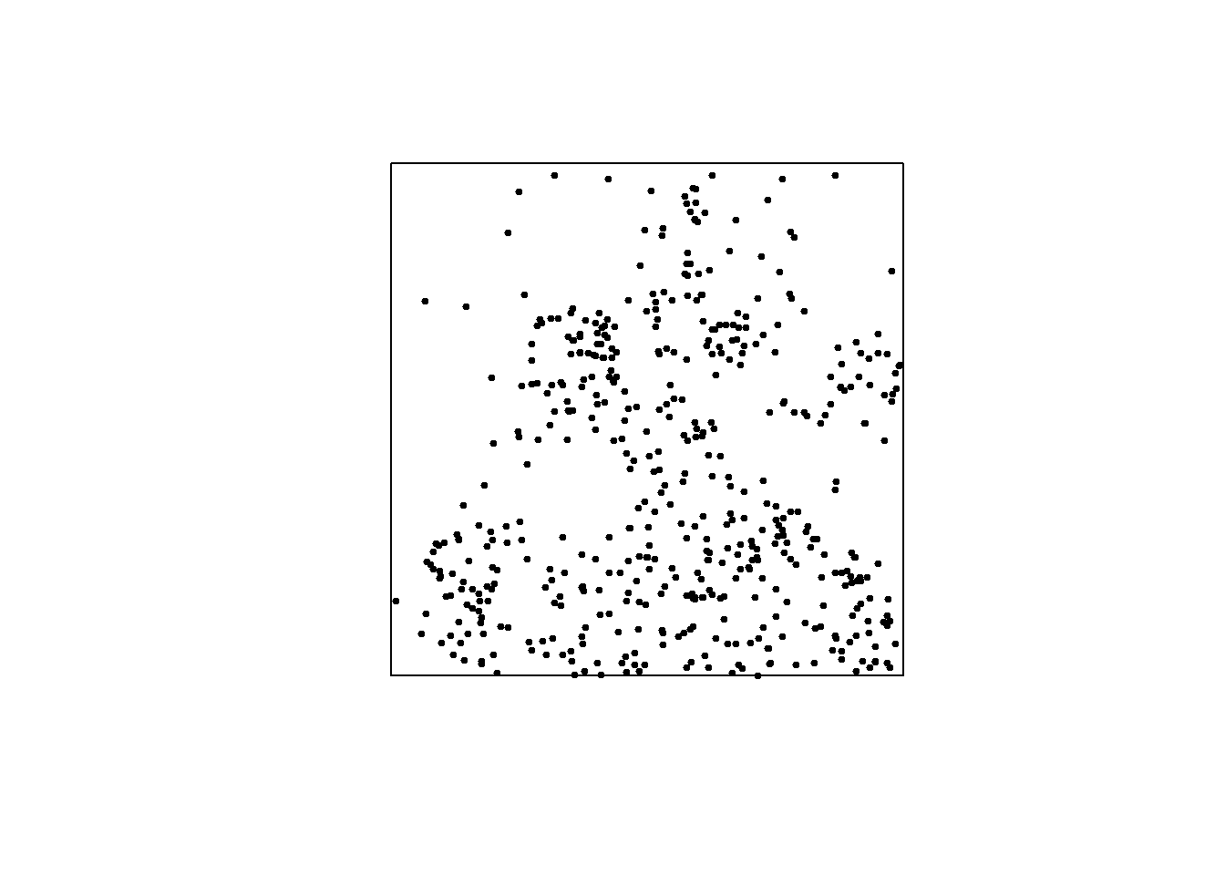
#log-likelihood
loglambda <- function(x, alpha, beta) {
   l <- alpha + sum(beta * c(x, x * x, prod(x)))
   return(l)
}

L <- function(alphabeta, x) {
   l <- apply(x, 1, loglambda, alpha = alphabeta[1], beta = alphabeta[-1])
   l <- sum(l)
   intL <- adaptIntegrate(lowerLimit = c(0, 0), upperLimit = c(1,1), fDim = 1, tol = 1e-08,
                f = function(x, alpha = alphabeta[1],beta = alphabeta[-1]){
           exp(loglambda(x, alpha, beta))})
   l <- l - intL$integral
   return(l)
}

#optimization
optbeta <- optim(par = c(log(nx), 0, 0, 0, 0, 0), fn = L,
                 control = list(maxit = 1000, fnscale = -1), x = x)

grd <- GridTopology(cellcentre.offset=c(0.005,0.005), cellsize=c(0.01, 0.01),
                    cells.dim=c(100, 100))
lambda<-exp(apply(coordinates(grd),1, function(X, alpha, beta)
{
  loglambda(X, alpha, beta)
}, alpha=optbeta$par[1], beta=optbeta$par[-1]
))
parint<-SpatialGridDataFrame(grd, data=data.frame(intensity=lambda))
lyt<-list("sp.points", SpatialPoints(x), pch=19, col="black", cex=0.7)
gp <- grey.colors(5, 0.9, 0.45, 2.2)

print(spplot(parint, at=seq(0,1400,length.out=8),
             col.regions=colorRampPalette(gp)(7), sp.layout=list(lyt)))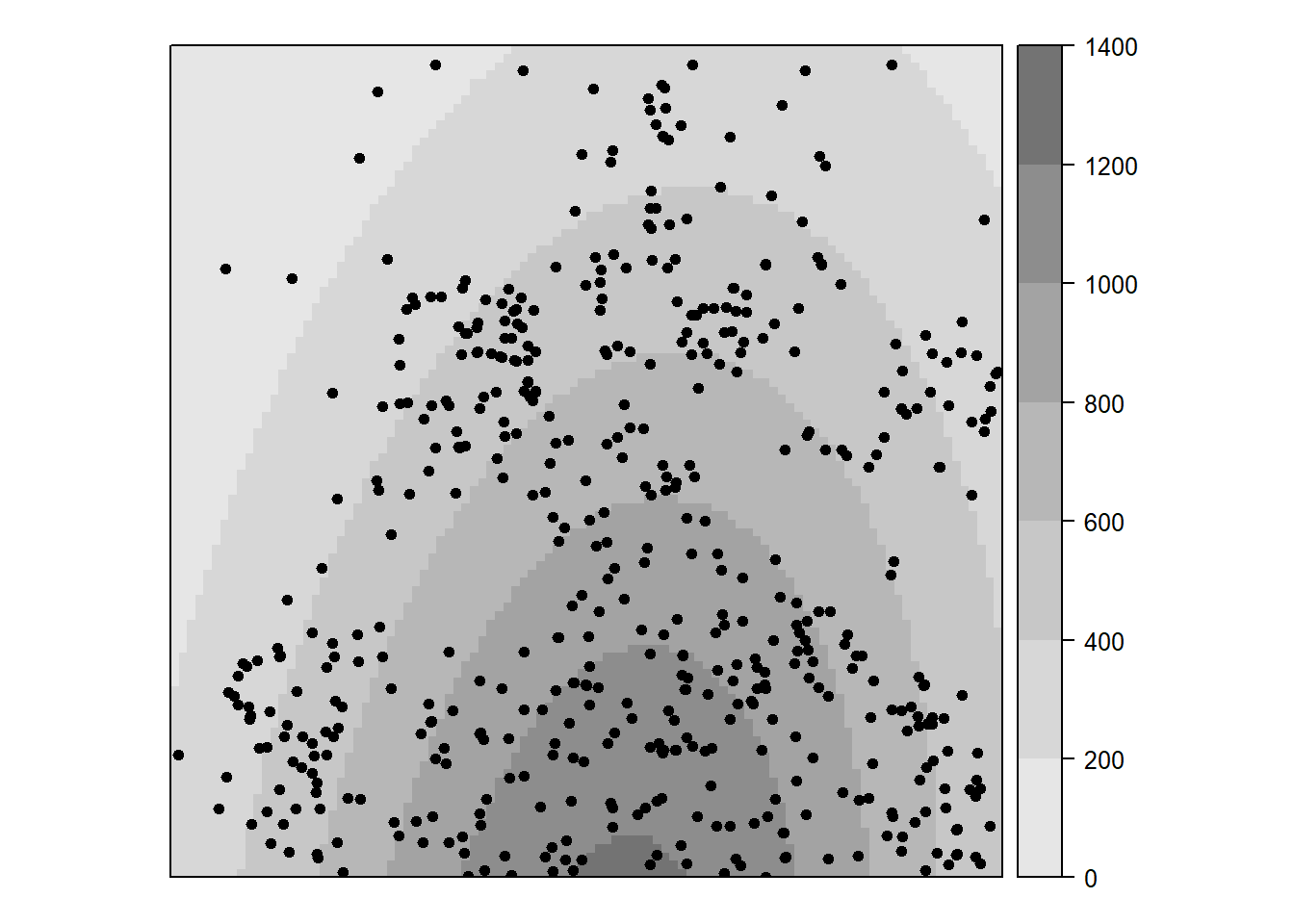
#using function "ppm" in spatstat package, we can do the estimation too.
library(spatstat)
lmaple <- lansing[lansing$marks == "maple", ]
ppm(Q = lmaple, trend = ~x + y + I(x^2) + I(y^2) + I(x * y))
## Nonstationary multitype Poisson process
##
## Possible marks: 'blackoak', 'hickory', 'maple', 'misc', 'redoak' and 'whiteoak'
##
## Log intensity: ~x + y + I(x^2) + I(y^2) + I(x * y)
##
## Fitted trend coefficients:
## (Intercept) x y I(x^2) I(y^2) I(x * y)
## 3.7311 5.6401 -0.7664 -5.0115 -1.1983 0.6376
##
## Estimate S.E. CI95.lo CI95.hi Ztest Zval
## (Intercept) 3.7311 0.2542 3.2329 4.22930 *** 14.6777
## x 5.6401 0.7990 4.0741 7.20608 *** 7.0589
## y -0.7664 0.6991 -2.1365 0.60375 -1.0963
## I(x^2) -5.0115 0.7012 -6.3858 -3.63726 *** -7.1474
## I(y^2) -1.1983 0.6428 -2.4582 0.06155 -1.8642
## I(x * y) 0.6376 0.6989 -0.7323 2.00743 0.9122Besag, Julian. 1974. “Spatial Interaction and the Statistical Analysis of Lattice Systems.” Journal of the Royal Statistical Society. Series B (Methodological). JSTOR, 192–236.
Besag, Julian, Jeremy York, and Annie Mollié. 1991. “Bayesian Image Restoration, with Two Applications in Spatial Statistics.” Annals of the Institute of Statistical Mathematics 43 (1): 1–20. doi:10.1007/BF00116466.
Bivand, Roger S, Edzer J Pebesma, Virgilio Gómez-Rubio, and Edzer Jan Pebesma. 2008. Applied Spatial Data Analysis with R. Vol. 747248717. Springer.
Cressie, N.A.C. 1993. Statistics for spatial data, 2nd ed. New York: Jone Wiley & Sons.
Diggle, Peter J. 2013. Statistical Analysis of Spatial and Spatio-Temporal Point Patterns. CRC Press.
Diggle, Peter J, JA Tawn, and RA Moyeed. 1998. “Model-Based Geostatistics.” Journal of the Royal Statistical Society: Series C (Applied Statistics) 47 (3). Wiley Online Library: 299–350.
Gelfand, A., P. Diggle, M. Fuentes, and P. Guttorp. 2010. Handbook of spatial statistics. CRC press.
Gelfand, Alan E, and Sujit K Ghosh. 1998. “Model Choice: A Minimum Posterior Predictive Loss Approach.” Biometrika 85 (1). Oxford University Press: 1–11.
Gelman, Andrew, John B Carlin, Hal S Stern, David B Dunson, Aki Vehtari, and Donald B Rubin. 2014. Bayesian Data Analysis. Vol. 2. CRC press Boca Raton, FL.
Kent, John T. 1989. “Continuity Properties for Random Fields.” Ann. Probab. 17 (4). The Institute of Mathematical Statistics: 1432–40. doi:10.1214/aop/1176991163.
Lahiri, Soumendra Nath, Yoondong Lee, and Noel Cressie. 2002. “On Asymptotic Distribution and Asymptotic Efficiency of Least Squares Estimators of Spatial Variogram Parameters.” Journal of Statistical Planning and Inference 103 (1). Elsevier: 65–85.
Ren, Qian, and Sudipto Banerjee. 2013. “Hierarchical Factor Models for Large Spatially Misaligned Data: A Low-Rank Predictive Process Approach.” Biometrics 69 (1). Wiley Online Library: 19–30.
Ripley, Brian D. 1977. “Modelling Spatial Patterns.” Journal of the Royal Statistical Society. Series B (Methodological). JSTOR, 172–212.
Schabenberger, Oliver, and Carol A Gotway. 2017. Statistical Methods for Spatial Data Analysis. CRC press.
Spiegelhalter, David J, Nicola G Best, Bradley P Carlin, and Angelika Van Der Linde. 2002. “Bayesian Measures of Model Complexity and Fit.” Journal of the Royal Statistical Society: Series B (Statistical Methodology) 64 (4). Wiley Online Library: 583–639.
Stein, Michael. 1999. Interpolation of spatial data: some theory for kriging. Springer.
References
Diggle, Peter J. 2013. Statistical Analysis of Spatial and Spatio-Temporal Point Patterns. CRC Press.
Ripley, Brian D. 1977. “Modelling Spatial Patterns.” Journal of the Royal Statistical Society. Series B (Methodological). JSTOR, 172–212.