Chapter 1 Introduction
1.1 The Need for spatial analysis
In a lot of statistical analysis, independence among observations is always assumed, which is an appropriate assumption for modeling independent data or weakly dependent data. However, it often fails for analyzing time series data, spatial data, and spatial-temporal data, where observations are correlated cross time, space, or both without independent replications.
For example, in a field study, \(\{(Y({\mathbf{s}}_i), X({\mathbf{s}}_i)), i=1,2,...,n\}\) were observed at locations \({\mathbf{s}}_1,...,{\mathbf{s}}_n\) in a given \(2D\) spatial domain. \(Y\) is the response variable and \(X\) is the predictor variable. In order to study the linear association between \(Y\) and \(X\), we may try a simple linear regression model \[ Y({\mathbf{s}}_i) = \beta_0 + \beta_1 X({\mathbf{s}}_i)+ \epsilon_{i}.\]
However, the usual assumption that \(\epsilon_i,i=1,...,n\) are independent is violated because of the spatial dependence. For example, when \(s_i\) and \(s_j\) are close to each other, \(Y\) and \(X\) are more likely to take similarly values. In this case, traditional estimation and inference on regression model cannot be applied to this setting directly. In the model diagnostics, the residual plot would show patterns. The regression models for those data should take care of explaining the special dependence structure.
Spatial models are applied to various of scientific areas, including Geology, agriculture, epidemiology, ecology, forestry, astronomy, atmospheric science, real estate, and any discipline that the spatial dependence among observations cannot be ignored in data analysis.
Spatial data vs. time series:
Time series are observed on time domain (one dimension); spatial data could be observed on \(1D\), \(2D\), or \(3D\) space. In general, it can be considered as data observed in \(d\)-dimensional space, where \(d\) is a positive integer.
Time flows in one direction only from past to present to future; it is not the case in space. So the dependence structure in spatial data could be more complicated.
Extrapolation (forecasting) is one of the main goals in time series analysis; interpolation is more meaningful in spatial analysis.
1.2 Types of Spatial Data
There are three types of spatial data.
- Geostatistical data (point referenced data):
Let \({\mathcal{D}}\) be a continuous domain in the \(d\)-dimensional Euclidean space \({\mathbb{R}}^d\). Let \(Y\) be the attribute/variable concerned in the study, such as temperature and PM2.5. The attribute \(Y\) can be measured everywhere in \({\mathcal{D}}\), that is between any two locations \({\mathbf{s}}_i\) and \({\mathbf{s}}_j\), theoretically there are infinite locations where \(Y\) are well defined. We end up using the spatial process \(\{Y({\mathbf{s}}), {\mathbf{s}}\in {\mathcal{D}}\}\) to model the attribute \(Y\) ( a collection of \(Y({\mathbf{s}})\) in \({\mathcal{D}}\)).
If data are collected at some locations \({\mathbf{s}}_1,...,{\mathbf{s}}_n\) in \({\mathcal{D}}\), say \(y({\mathbf{s}}_1), y({\mathbf{s}}_2), ..., y({\mathbf{s}}_n)\), the dataset is called geostatistical data or point referenced data.
- Lattice data (regional data or areal data) Let \({\mathcal{S}}=\{A_i\subset {\mathbb{R}}^d, i=1,2,...\}\) be a discrete/countable domain in \(d\)-dimensional Euclidean space \({\mathbb{R}}^d\). The attribute \(Y\) could be measured at any areal regions in \({\mathcal{S}}\), but not any point in space. For example, \(Y\) can be ZIP code, prime rate of a county, or remotely sensed data reported by pixels. So we can use a spatial process \(\{Y(A_i), A_i\in {\mathcal{S}}\}\) to model the attribute \(Y\). Spatial locations in such process are often referred to as sites。
For the notation convenience, in the following, while considering lattice data, we may still use \(\{Y({\mathbf{s}}), {\mathbf{s}}\in {\mathcal{D}}\}\) to represent lattice data. If so, please notice that the location \({\mathbf{s}}\) represents an areal region \(A_i\) and the domain \({\mathcal{D}}\) denotes the countable discrete set \({\mathcal{S}}\) defined above.
If data are collected on some sites \({\mathbf{s}}_1,...,{\mathbf{s}}_n\) in \({\mathcal{D}}\), say \(y({\mathbf{s}}_1), y({\mathbf{s}}_2), ..., y({\mathbf{s}}_n)\), the dataset is called lattice data, regional data or areal data.
Remark: The distinction between geostatistical data and lattice data are not always clearcut. For example, the remote sensing data with very low resolution can be considered as lattice data; the remote sensing data with very high resolution can be considered as geostatistical data; those with moderate resolution could be considered as either one, determined by the goal of the study.
- Point Patterns: Point patterns arise when the important variable to be analyzed is the location of events. The first question to ask is whether the pattern is exhibiting complete spatial randomness, clustering, or regularity (see, e.g., N. Cressie (1993)). For example, locations of avian flu over the world, locations of long leaf pines in a natural forest. So for spatial point pattern data, the randomness is the spatial locations in a given domain. The formal definition of spatial point process will be given later.
Moreover, if some other variable is considered on those locations, it is called marked variable. For example, if we also measure the diameters of the long leaf pines, the point pattern together with the marked variable is called a marked spatial point process.
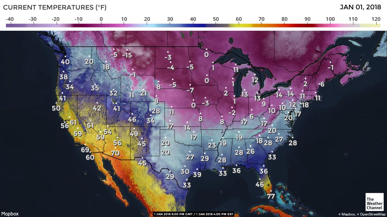
Example 1.1 (Arctic Outbreak) “Arctic air has returned to the Lower 48 and will keep frigid conditions in place across the nation’s northern tier into at least the first few days of 2018”. See details in https://weather.com/forecast/national/news/2017-12-18-arctic-cold-outbreak-forecast-christmas-2017.
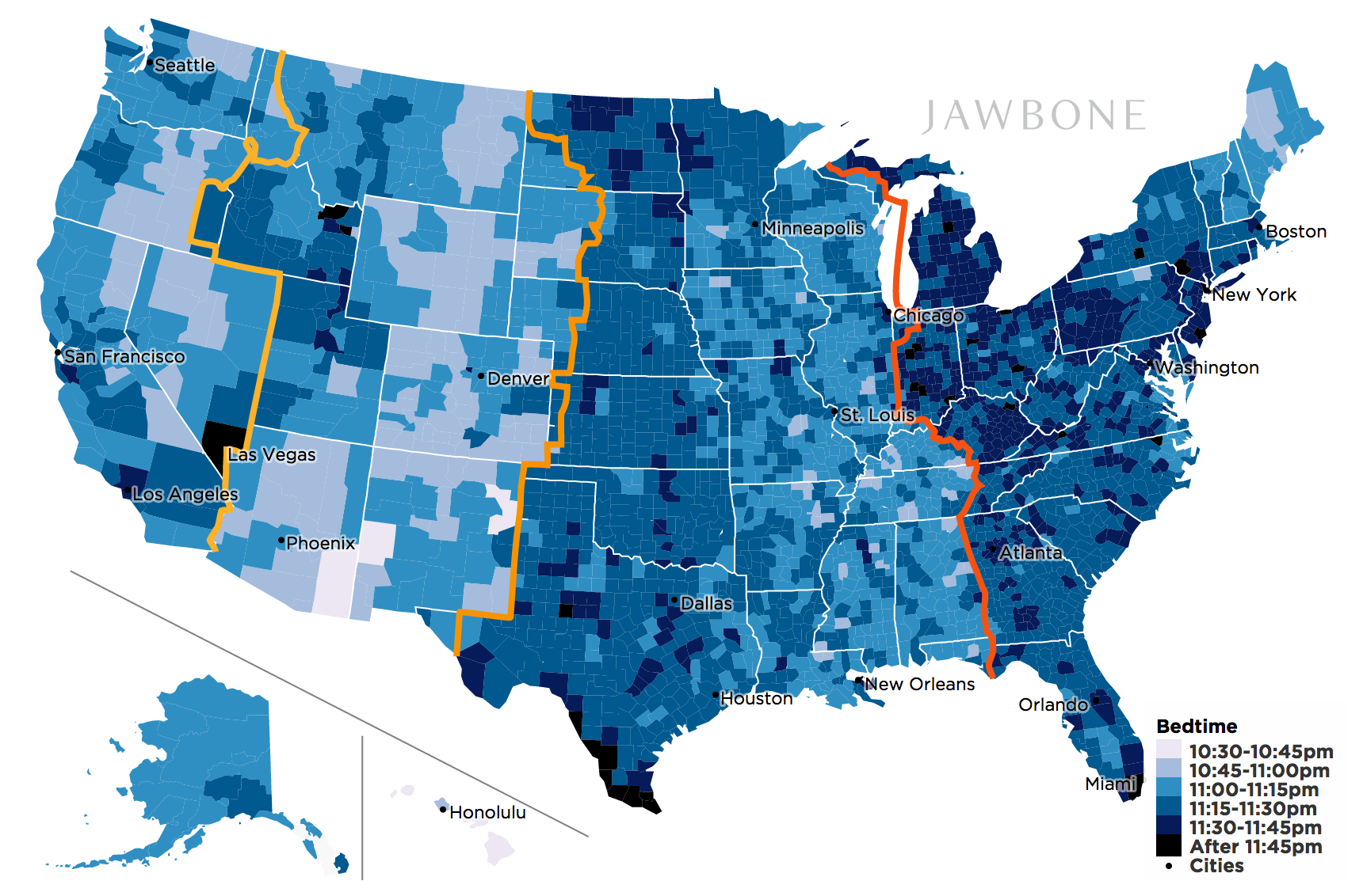
Example 1.2 (Bed time) In which counties people go to bed early? The following plot was copied from https://jawbone.com/blog/circadian-rhythm/.

1.3 The Effects of Spatial Dependence on Statistical Inference and Predictions
Here, we provide two examples to explain the effect of spatial dependence, and how the inference and predictions could be improved when the spatial dependence structure is utilized.
\[\begin{equation} \begin{split} & Y_i = \mu + \epsilon_i, \\ & \epsilon_i \sim N(0,\sigma^2), \\ & \text{Cov}(\epsilon_i, \epsilon_j) = \sigma^2 \rho^{|i-j|}, \end{split} \tag{1.1} \end{equation}\] where \(i, j = 1, ..., n\), \(\sigma^2 > 0\) and \(\rho \in (0,1)\). For simplicity, suppose that \(\sigma^2\) and \(\rho\) are known. Will the sample mean a good estimator for \(\mu\)? If not, any alternatives?
Solution. 1. The sample mean is an unbiased estimator. \[{\mathbb{E}}(\bar Y) = \frac{1}{n} \sum_{i=1}^n {\mathbb{E}}(Y_i) = \mu.\]
- To evaluate the efficiency of the estimator, consider the variance of the sample mean
Since for \(\rho \in (0,1)\), \(C(\rho, n) > 1\) and hence \(\text{Var}(\bar{Y}) > n^{-1} \sigma^2\). As we know, if \(Y_1, ..., Y_n\) are independent with each other, the variance of \(\bar Y\) is \(n^{-1} \sigma^2\). So we can see that sample mean for correlated data seems not as efficient as that for independent data.
Further, if we consider the 95% confidence interval for \(\mu\). The Z interval is given by \[ \bar Y \pm 1.96 sd(\bar Y) = \bar Y \pm 1.96 \frac{\sigma\sqrt{C(\rho,n)}}{\sqrt{n}} .\] So it is wider than the case when \(Y_i\)s are independent. With the same accuracy, the equivalent number of observations needed in the independent case, so called effect sample size is given by \(n' = n/C(\rho,n).\)
The following shows how \(n'\) changes with \(\rho\) given \(n=50\). 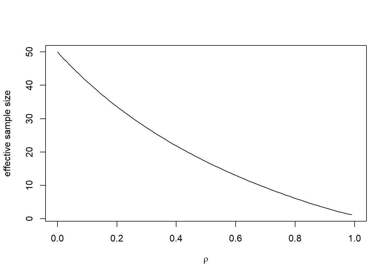
- Any alternative estimator to improve the efficiency of estimating \(\mu\)?
Let \({\mathbf{Y}}=(Y_1, ..., Y_n)^\top\), \(\text{Var}({\mathbf{Y}}) = \Sigma\), and \({\boldsymbol{\epsilon}}= (\epsilon_1, ..., \epsilon_n)^\top\). Then the matrix form of the above model is \[{\mathbf{Y}}= \mathbf{1}\mu + {\boldsymbol{\epsilon}}.\] Here, \(\Sigma\) has an explicit inverse, that is \[\Sigma^{-1} = \frac{1}{\sigma^2(1-\rho^2)}\begin{pmatrix} 1 & -\rho &0 &0 &\cdots & 0\\ -\rho & 1+\rho^2 & -\rho& 0 &\cdots & 0\\ 0 & -\rho & 1+\rho^2 & -\rho &\cdots & 0\\ 0 & 0&-\rho & 1+\rho^2 & \cdots & \vdots\\ \vdots & \vdots &\vdots &\cdots &\ddots &-\rho\\ 0&0&\cdots&0&-\rho&1 \end{pmatrix}\]
Let \[C_{GLS}(n,\rho) = \frac{n(1+\rho)}{(n-2)(1-\rho)+2},\ \text{and}\ w_1=w_n=\frac{C_{GLS}(n,\rho)}{n(1+\rho)}, w_2=\cdots=w_{n-1}=\frac{C_{GLS(n,\rho)}}{n}.\]
The generalized least square estimator of \(\mu\) is given by \[\hat \mu_{GLS} = (\mathbf{1}^\top \Sigma^{-1}\mathbf{1})^{-1}(\mathbf{1}^\top \Sigma^{-1}{\mathbf{Y}})=\sum_{i=1}^n w_i Y_i,\] and the variance of \(\hat \mu_{GLS}\) is \[\text{Var}(\hat \mu_{GLS}) = (n^{-1}\sigma^2)C_{GLS}(n,\rho).\]
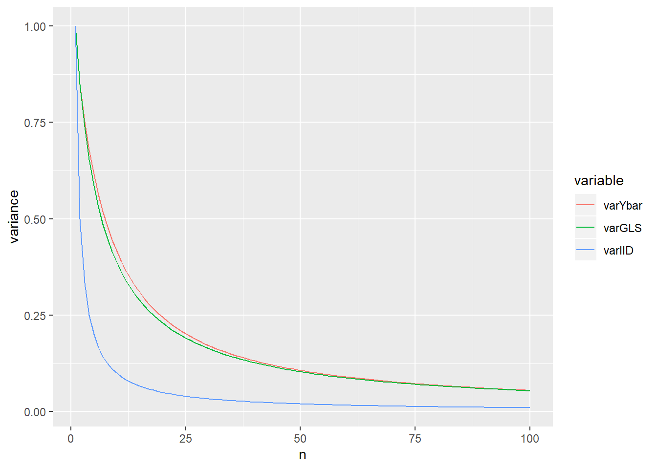
Indeed, \(\hat \mu\) is the best linear unbiased estimator (BLUE). The following shows how the efficiency of \(\bar Y\) and \(\hat \mu_{GLS}\) changes with \(\rho\) given \(n=30\). 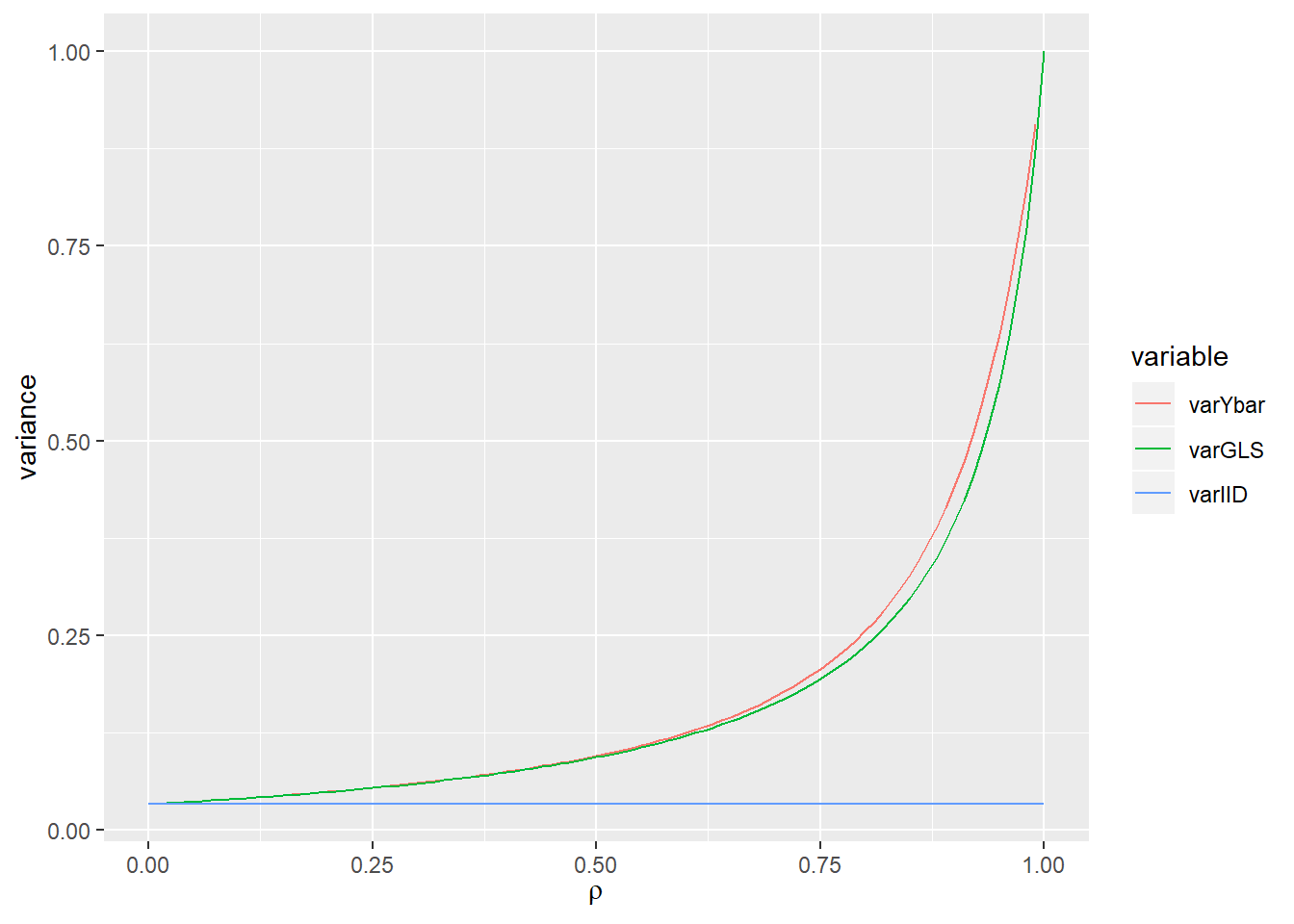
Given \(\rho = 0.7\), the following shows how the efficiency of \(\bar Y\) and \(\hat \mu_{GLS}\) changes with \(n\) increasing.
Solution. 1. Let \({\mathbf{a}}= (a_1, ..., a_n)^\top\) be \(n\)-dimensional vector and the linear prediction of \(Y_0\) can be written as \[\hat Y_0 = \sum_{i=1}^n a_i Y_i = a^\top {\mathbf{Y}}.\]
Since \(\hat Y_0\) is required to be unbiased, it should satisfy \[{\mathbb{E}}(\hat Y_0) = \mu.\] Hence, \[{\mathbf{a}}^\top {\mathbb{E}}({\mathbf{Y}}) = {\mathbf{a}}^\top \mathbf{1}\mu = \mu\] which leads to a restriction on \({\mathbf{a}}\), \[{\mathbf{a}}^\top \mathbf{1} = 1, \ \ \text{i.e.,} \ \sum_{i=1}^n a_i = 1.\]
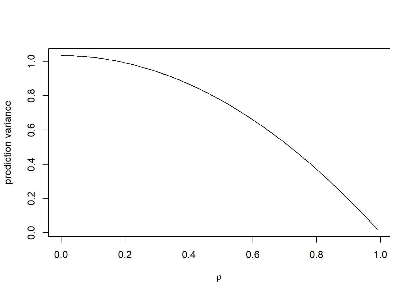
In order to find the best linear unbiased prediction, we should minimize \[{\mathbb{E}}({\mathbf{a}}^\top {\mathbf{Y}}- Y_0)^2\ \ \text{subject to}\ \ a^\top \mathbf{1} = 1.\] The solution is \[\hat Y_0 = \hat \mu_{GLS} + {\mathbf{c}}^\top \Sigma^{-1}({\mathbf{Y}}-\mathbf{1}\hat \mu_{GLS}).\] Further, we can obtain the variance of \(\hat Y_0\), \[\sigma_{pred}^2 = {\mathbb{E}}(\hat Y_0-Y_0)^2 = \sigma^2 - {\mathbf{c}}^\top \Sigma^{-1}{\mathbf{c}}+ (1-\mathbf{1}^\top \Sigma^{-1}{\mathbf{c}})^2(\mathbf{1}^\top \Sigma^{-1}\mathbf{1})^{-1}=\sigma^2(1+1/n)C(n,\rho),\] where \[C(n,\rho) = (1-\rho^2)\left\{1-\frac{2\rho}{(n+1)(n-n\rho+2\rho)}\right\}\leq 1-\rho^2\leq 1, \ \text{for}\ \rho \in [0,1].\]
Summary:
With spatial dependence, the generalized least square estimator of a single mean, which utilizes the dependence structure are more efficient than the sample mean estimator.
With spatial dependence, even the GLS estimator has higher variability than that of independent data. In other words, with the same sample size, estimating mean structure with dependent data is less accurate.
With spatial dependence, the prediction error of variables at a new location may be smaller than that with independent data.
References
Cressie, N.A.C. 1993. Statistics for spatial data, 2nd ed. New York: Jone Wiley & Sons.