Chapter 4 Statistics Modeling of Lattice data (Discrete spatial variation)
In this chapter, we’ll consider statistical models for lattice data (areal data). Recall that lattice data can be considered as a partial realization of spatial random field \(\{ Y(\mathbf{s}), \mathbf{s}\in {\mathcal{D}}\}\), where the index set \({\mathcal{D}}\) is a countable spatial sites (or regions) at which data are observed.
4.1 Exploratory Data analysis and visualization
rm(list=ls())
library(spdep)
library(rgdal)
library(RColorBrewer)
library(classInt)

nc.sids <- readOGR(system.file("shapes/sids.shp", package="spData")[1], verbose = FALSE)
proj4string(nc.sids) <- CRS("+proj=longlat +ellps=clrk66")
brks = c(0, 5, 10, 20, 30, 57)
color.pallete = rev(brewer.pal(5,"RdBu"))
class.SID79 = classIntervals(var=nc.sids$SID79, n=5, style="fixed",fixedBreaks=brks)
class.SID74 = classIntervals(var=nc.sids$SID74, n=5, style="fixed",fixedBreaks=brks)

color.code.SID79 = findColours(class.SID79, color.pallete)
color.code.SID74 = findColours(class.SID74, color.pallete)

plot(nc.sids, col=color.code.SID74)
title("SID deaths 1974-1978" )
leg.txt = c(paste("<",brks[2], sep=""),
            paste(brks[2],"-", brks[3]-1, sep = ""),
            paste(brks[3], "-", brks[4]-1, sep = " "),
            paste(brks[4], "-", brks[5], sep = ""),
            paste(">", brks[5], sep = " "))
legend("bottomleft", legend=leg.txt, cex=1, bty="n", horiz = FALSE, fill = color.pallete)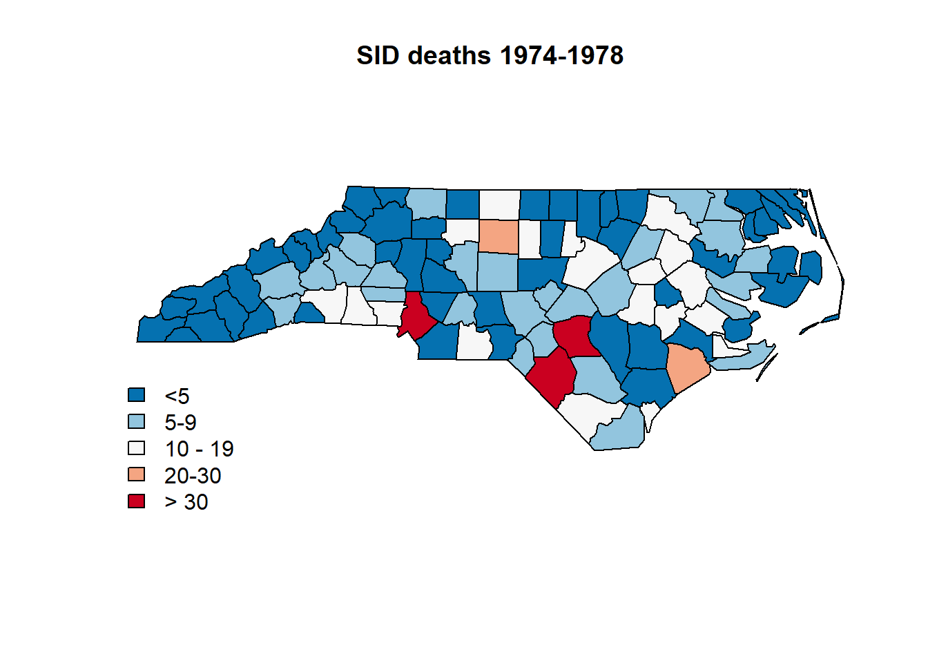
plot(nc.sids, col=color.code.SID79)
title("SID deaths 1979-1984" )
legend("bottomleft", legend=leg.txt, cex=1, bty="n", horiz = FALSE, fill = color.pallete)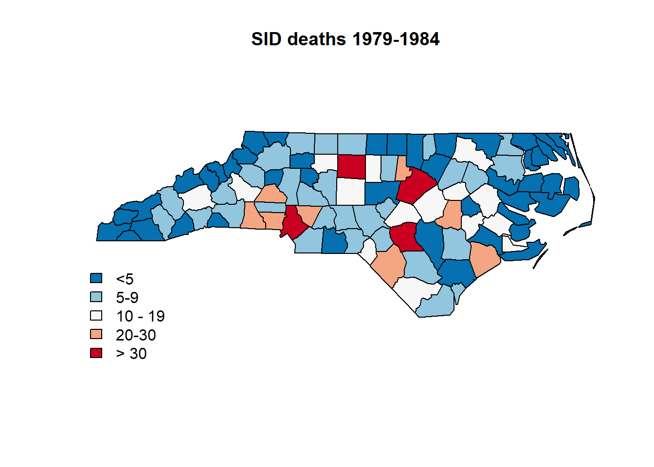
4.1.1 Proximity matrix
We first introduce the concept of proximity matrix (spatial-neighborhood matrix) \(W\). Given lattice data \(y({\mathbf{s}}_1), ..., y({\mathbf{s}}_n)\), the entries \(w_{ij}\) in \(W\) spatially connect sites \({\mathbf{s}}_i\) and \({\mathbf{s}}_j\). If site \({\mathbf{s}}_j\) is considered as “neighbor” of \({\mathbf{s}}_i\), then \(w_{ij}=1\); otherwise, \(w_{ij} = 0\). Usually, \(w_{ii}\) is set to zero.
The definition of the “neighbor” of a site is made by the modeler. For example, any site who shares some common boundary, perhaps a vertex (as in a regular grid) with the site \({\mathbf{s}}_i\), can be considered as a neighbor of \({\mathbf{s}}_i\). Or we can define any sites within some specific distance from \({\mathbf{s}}_i\) as the neighbors of \({\mathbf{s}}_i\). Or we can choose the nearest \(K\) sites (in distance) of \({\mathbf{s}}_i\) as its neighbors.
From the definition, we can see that the \(i\)th row of \(W\) label all sites that are “close” to the site \({\mathbf{s}}_i, i=1,...,n\) as \(1\).
Here is an example of how to extract the proximity matrix of county data in R.rm(list=ls())
library(maps)
library(maptools)
map.text("county", "nebraska", fill = FALSE, plot = TRUE, cex = 0.5)
ne.county = map("county", "nebraska", fill = TRUE, plot = FALSE)
county.ID <- sapply(strsplit(ne.county$names, ","), function(x) x[2])
ne.poly = map2SpatialPolygons(ne.county, IDs=county.ID)
ne.nb = poly2nb(ne.poly)
ne.adj.mat = nb2mat(ne.nb, style="B")

#find neighbors of Lancaster county in Nebraska
ne.region.id <- attr(ne.nb, "region.id")
lancaster.neighbors.index = ne.nb[[match("lancaster", ne.region.id)]]
lancaster.neighbors = rownames(ne.adj.mat[lancaster.neighbors.index,])
lancaster.neighbors
## [1] "butler" "cass" "gage" "johnson" "otoe" "saline" "saunders"
## [8] "seward"4.1.2 Measures of Spatial Association (Moran’s I and Geary’s C)
Two tests that are used to measure the strength of spatial association among lattice data are Moran’s I test and Geary’s C test, which test whether the lattice data are independent or not. The tests are constructed by assuming the lattice data model has constant mean and variance.
For simplicity, let \(y_i = y({\mathbf{s}}_i)\) and let \(\bar y = \frac{1}{n}\sum_{i=1}^n y_i\).
Moran’s I statistic is defined as \[I = \frac{n\sum_{i,j=1}^n w_{ij}(y_i -\bar y)(y_j-\bar y)}{(\sum_{i\neq j} w_{ij})\sum_{i=1}^n (y_i-\bar y)^2}.\] Under the null model where \(y_i\)s are i.i.d. (independent and identically distributed), \(I\) is asymptotically normally distributed with mean \({\mathbb{E}}(I) = -1/(n-1)\). If \(I > {\mathbb{E}}(I)\), then the neighbors of the site \({\mathbf{s}}_i\) tend to have similar \(y\) values as \(y({\mathbf{s}}_i)\); if \(I < {\mathbb{E}}(I)\), then the neighbors of the site \({\mathbf{s}}_i\) tend to have dissimilar \(y\) values as \(y({\mathbf{s}}_i)\).
Since the Moran’s I is sensitive to changes in the mean function, we recommend the use of Moran’s I as exploratory measure of spatial association rather than as a “test of spatial significance”.
Although Moran’s I converges to Gaussian distribution as sample size \(n\) goes to infinity, the speed of convergence is low. For small or moderate sample size \(n\), permutation test or Monte Carlo test is preferred.
Permutation test: Under null hypothesis, \(y({\mathbf{s}}_1), ..., y({\mathbf{s}}_n)\) can be thought of as a random assignment of values to sites \({\mathbf{s}}_1, ..., {\mathbf{s}}_n\). With \(n\) sites, the number of possible assignments is \(n!\). For each assignment, we can calculate one \(I\) and hence we get the distribution of \(I\) under null hypothesis. The p value of the test can be calculated by the probability of \(I\) being as extreme as the observed \(I\).
Monte Carlo test: Even for moderately large \(n\), the number of possible assignments \(n!\) is large. Instead of a complete enumeration, one can sample independently \(k\) random assignments to construct the empirical null distribution of \(I\). Then an empirical p value of the test can be calculated.
Geary’s C statistic is defined as \[ C = \frac{(n-1)\sum_{i,j=1}^n w_{ij}(y_i - y_j)^2}{(\sum_{i\neq j} w_{ij})\sum_{i=1}^n (y_i-\bar y)^2}.\] \(C\) is non-negative. Under the null model where \(y_i\)s are i.i.d. (independent and identically distributed), \(C\) is asymptotically normally distributed with mean \({\mathbb{E}}(C) = 1\). That \(C < 1\) indicates positive spatial association.
Similarly as Moran’s I test, we recommend the use of Geary’s C as exploratory measure of spatial association rather than as a “test of spatial significance”. Also, rather than using z test, we use permutation test or Monte Carlo test to compute the p value.
We can use “moran.test” and “geary.test” in R to measure the spatial association of SIDS data in Example 4.1.
rm(list=ls())
library(spdep)
library(rgdal)
library(RColorBrewer)
library(classInt)

nc.sids <- readOGR(system.file("shapes/sids.shp", package="spData")[1], verbose = FALSE)
proj4string(nc.sids) <- CRS("+proj=longlat +ellps=clrk66")
#get the proximity matrix
row.names(nc.sids) <- as.character(nc.sids$FIPS) #FIPS County ID
rn <- row.names(nc.sids)
ncCC89.nb <- read.gal(system.file("weights/ncCC89.gal", package="spData")[1],
                      region.id=rn)
plot(nc.sids, border="grey")
plot(ncCC89.nb, coordinates(nc.sids), add=TRUE, col="blue")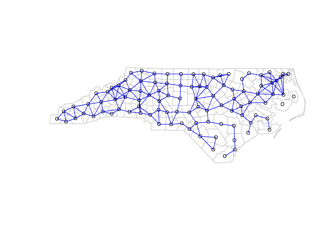
#compute Moran's I and Geary's C
ncCC89.listw = nb2listw(ncCC89.nb, style="B", zero.policy=TRUE)
nc.sids74.moran.out = moran.test(nc.sids$SID74, listw=ncCC89.listw, zero.policy=TRUE)
nc.sids74.moran.out
##
## Moran I test under randomisation
##
## data: nc.sids$SID74
## weights: ncCC89.listw n reduced by no-neighbour observations
##
##
## Moran I statistic standard deviate = 2.0994, p-value = 0.01789
## alternative hypothesis: greater
## sample estimates:
## Moran I statistic Expectation Variance
## 0.129486557 -0.010309278 0.004433961nc.sids74.geary.out = geary.test(nc.sids$SID74, listw=ncCC89.listw, zero.policy=TRUE)
nc.sids74.geary.out##
## Geary C test under randomisation
##
## data: nc.sids$SID74
## weights: ncCC89.listw
##
## Geary C statistic standard deviate = 1.9867, p-value = 0.02348
## alternative hypothesis: Expectation greater than statistic
## sample estimates:
## Geary C statistic Expectation Variance
## 0.73930443 1.00000000 0.01721963nc.sids79.moran.out = moran.test(nc.sids$SID79, listw=ncCC89.listw, zero.policy=TRUE)
nc.sids79.moran.out##
## Moran I test under randomisation
##
## data: nc.sids$SID79
## weights: ncCC89.listw n reduced by no-neighbour observations
##
##
## Moran I statistic standard deviate = 2.8735, p-value = 0.00203
## alternative hypothesis: greater
## sample estimates:
## Moran I statistic Expectation Variance
## 0.181462985 -0.010309278 0.004454068nc.sids79.geary.out = geary.test(nc.sids$SID79, listw=ncCC89.listw, zero.policy=TRUE)
nc.sids79.geary.out##
## Geary C test under randomisation
##
## data: nc.sids$SID79
## weights: ncCC89.listw
##
## Geary C statistic standard deviate = 2.0151, p-value = 0.02195
## alternative hypothesis: Expectation greater than statistic
## sample estimates:
## Geary C statistic Expectation Variance
## 0.73969349 1.00000000 0.016686674.2 Modeling Lattice data
One way to model the lattice data \(y({\mathbf{s}}_1), ..., y({\mathbf{s}}_n)\) with spatial dependence is to construct a \(n\) dimensional joint density distribution, say \(p(y_1,...,y_n)\). For continuous and symmetric lattice data, we can model it using multivariate Gaussian distribution. For skewed or discrete data, we can use distributions from exponential families.
Yet, unlike the geostatistical data, the covariance of \(y({\mathbf{s}}_1), ..., y({\mathbf{s}}_n)\) is usually not defined by a covariance function \(C({\mathbf{s}},{\mathbf{s}}';{\boldsymbol{\theta}})\). Rather, a Markov type of spatial dependence structure is widely applied in practice. In this section, we’ll first introduce the main theories to construct lattice data model, that are Brook’s Lemma and Markov random fields. Then, we introduce Conditionally autoregressive (CAR) models.
4.2.1 Brook’s Lemma and Markov random fields
It is clear that given the joint density \(p(y_1,...,y_n)\), the full conditional distributions, \(p(y_i\,|\, y_1,..,y_{i-1},y_{i+1},...,y_n), i = 1,2,...,n\) are uniquely determined.
Then, if we specify each of the full conditional \(p(y_i\,|\, y_1,..,y_{i-1},y_{i+1},...,y_n), i = 1,2,...,n\), can we obtain a unique joint density \(p(y_1,...,y_n)\)? If so, the distribution of lattice data can be modeled via its full conditional distributions.
Brook’s Lemma demonstrates it.
When the number of area units (regions) is large, we do not seek to write down the joint distribution of \((y({\mathbf{s}}_1),...,y({\mathbf{s}}_n))\). Rather we prefer to model the \(n\) full conditional distributions. It works very well especially in spatial lattice data, since the full conditional distributions can further be simplified to only depend on the neighbors of the site. The proximity (neighborhood) matrix \(W\) defined in the previous section provides all the “neighbors” information for lattice data. Let \(\partial_i\) denote the set of neighbors of site \({\mathbf{s}}_i\) and let \(\mathbf{y}_{-i} = (y_1,..,y_{i-1}, y_{i+1},y_n)\). Now for \(i=1,...,n\), we specify the full conditional distribution of \(y({\mathbf{s}}_i)\) by \[p(y_i\,|\, \mathbf{y}_{-i}) = p(y_i\,|\, y_j, j\in \partial_i).\] If a spatial lattice process \(\{Y({\mathbf{s}}), {\mathbf{s}}\in {\mathcal{D}}\}\) satisfies the above specification, we call it Markov random field.
Now the critical question is what kind of lattice process have the “Markov” type property? Here we need some new definitions.
The proximity (spatial neighborhood) matrix for lattice data can also been represented by a graph \({\mathcal{G}}= ({\mathcal{V}}, {\mathbb{E}})\), where \({\mathcal{V}}=\{{\mathbf{s}}_1,...,{\mathbf{s}}_n\}\), and \({\mathcal{E}}\) includes all edges of the graph. If \(s_j\) is the “neighbor” of \({\mathbf{s}}_i\), then there is an edge between \(s_j\) and \(s_i\). Some of the subgraphs of \({\mathcal{G}}\) should be cliques. The following Hammersley-Clifford theorem states the general form of joint distribution of a Markov random field.
Applying the above theorem, we can construct varies of valid joint densities for Markov random fields.
Example 4.3 For continuous lattice data, a choice for the joint distribution is a pairwise difference form,
\[p(y_1,...,y_n) \propto \exp\left(-\frac{1}{2\tau^2}\sum_{i\sim j} (y_i-y_j)^2 \right),\] where \(i\sim j\) means the pair of sites \(({\mathbf{s}}_i,{\mathbf{s}}_j)\) are mutual neighbors.
Its full conditional distributions are \[p(y_i \,|\, y_{-i}) \sim Gaussian(\sum_{j\in \partial_i} y_j/m_i, \tau^2/m_i),\] where \(m_i\) is the number of neighbors of site \(s_i\).Example 4.4 (Binary Markov random field) Consider binary lattice data in \(2D\) domain. The joint distribution can be modeled as
\[p(y_1,...,y_n) \propto \exp\left(\psi \sum_{i\sim j}w_{ij} (y_iy_j+ (1-y_i)(1-y_j))\right),\] where \(w_{ij} = w_{ji}\). The parameters \(w_{ij}\) control the interaction. This density is always valid since it cat take on only \(2^n\) values. However, it is not easy to calcualte the normalizing constant of the density since it needs summation over all \(2^n\) possible values of \(\mathbf{y}\).
We can get the full conditional distributions \[p(y_i=1 \,|\, y_{-i}) = \frac{e^{\psi m_{i,1}}}{e^{\psi m_{i,0}}+e^{\psi m_{i,1}}},\] where \(m_{i,1}\) is the number of neighbors of \(s_i\) that are equal to \(1\) and \(m_{i,0}\) is the number of neighbors of \(s_i\) that are equal to \(0\). Further,
\[logit(p(y_i=1 \,|\, y_{-i})) = (m_{i,1}-m_{i,0})\psi.\] If we bring in predictors to the above models, then \[logit(p(y_i=1 \,|\, y_{-i})) = (m_{i,1}-m_{i,0})\psi + \mathbf{X}_i^\top {\boldsymbol{\beta}},\] which is called autologistic CAR model for lattice data.4.2.2 Conditionally autoregressive (CAR) models
The conditionally autoregressive (CAR) models were introduced by Besag (1974) 44 years ago. There is a dramatic increase in applications in the past decade or so.
We first introduce auto Gaussian CAR model.
Consider a set of lattice data \({\mathbf{y}}= (y_1,...,y_n)\), which were observed at sites \({\mathbf{s}}_1,...,{\mathbf{s}}_n\). Let \(W\) be a symmetric proximity (spatial neighborhood) matrix. \(w_{ij}\) is set to zero if site \(i\) and \(j\) are neighbors; otherwise, \(w_{ij}=0\). Let the \(i\)th row sum of the matrix \(W\) be \(w_{i+} = \sum_{j=1}^n w_{ij}\). We can use \(W\) to rewrite the model introduced in Example 4.3 as \[p({\mathbf{y}}) = p(y_1,...,y_n) \propto \exp\left(-\frac{1}{2\tau^2}\sum_{i,j=1}^n w_{ij}(y_i-y_j)^2 \right) = \exp\left(-\frac{1}{2\tau^2}{\mathbf{y}}^\top(D_w -W){\mathbf{y}}\right),\] where \(D_w\) is diagonal matrix with \((D_w)_{ii} = w_{i+}\).
The full conditionals of the above joint density are given by \[p(y_i \,|\, y_{-i}) \sim Gaussian(\sum_{j} w_{ij}y_{j}w_{i+}, \tau^2/w_{i+}).\] The above model is called intrinsically autoregressive (IAR) model.
Remark:
i). The precision matrix (the inverse of the covariance matrix) of the above model is \[\Sigma_y^{-1} = \frac{1}{\tau^2}(D_w -W).\] It is singular since \((D_w - W)\mathbf{1} = \mathbf{0}\) and hence the joint density is not proper (integration of \(p({\mathbf{y}})\) is not equal to 1).
ii). Adding any constant to all of the \(y_i\) would provide the same value of \(p({\mathbf{y}})\). A restriction on \(\sum_i y_i = 0\) is necessary for centering.
iii). Due to the impropriety of \(p({\mathbf{y}})\), the joint density \(p({\mathbf{y}})\) above cannot be used to model the data directly. However, the full conditionals of \(p({\mathbf{y}})\) are valid densities, hence the IAR model is still used to model the spatial random effect in hierarchical models.
In order to fix the problem of improper \(p({\mathbf{y}})\), one way is to adding a parameter \(\rho \in (-1,1)\) and get the so-called Gaussian conditional autoregressive model (CAR) model,
\[p({\mathbf{y}}) = p(y_1,...,y_n) \propto \exp\left(-\frac{1}{2\tau^2}{\mathbf{y}}^\top(D_w -\rho W){\mathbf{y}}\right).\]
The full conditionals of the above joint density are given by \[p(y_i \,|\, y_{-i}) \sim Gaussian(\rho\sum_{j} w_{ij}y_j/w_{i+}, \tau^2/w_{i+}).\]
Remark:
i). By adding \(\rho\) to IAR model, the resulting CAR model has positive definite precision matrix \(\Sigma_y^{-1}\) and the joint density is proper. Hence, CAR model can be used to directly model lattice data \({\mathbf{y}}\).
ii). The additional \(\rho\) enriches the class of spatial model. When \(\rho =0\), it is reduced to independent model, that is \(y_i\)s are independent and follows Gaussian distribution with mean zero and variance \(\tau^2/w_{i+}\). Besides, by the theory of Gaussian Markov random fields, \[{\text{Cov}}(y_i,y_j \,|\, y_k, k \neq i,j) = \frac{\tau^2 \rho w_{ij}}{w_{i+}w_{j+} + \rho^2 w_{ij}^2}.\]
iii). Does \(\rho\) produce any problem in terms of model interpretation? Probably yes. For example, in an IAR model, the mean of \(y_i\) is considered as an average of its neighbors. However, in a CAR model, it is equal to some proportion of the average of its neighbors.
iv). Model parameter estimations can be implemented by maximum likelihood estimations or Bayesian MCMC methods.
Now we apply CAR model to SIDS data. Rather looking at the number of SIDs, we want to model the ratio between and SIDs and the total number of live births. Define the SID rate as \[w_i = 1000(s_i+1)/n_i,\] where \(s_i\) is the number of SIDs in county \(i\) and \(n_i\) the number of live births in county \(i\). The number of SIDs \(s_i\) follows binomial distribution, so \[{\mathbb{E}}(s_i/n_i) = p_i\ \text{and}\ {\text{Var}}(s_i/n_i) = p_i(1-p_i)/n_i.\] For small \(p_i\), the variance is proportional to the mean, suggesting a square-root transformation to remove this mean-variance dependence. However, it is more likely that the \(s_i\)s are spatially dependent Binomial random variables, in which case a severe transformation may be necessary. We can use Freeman-Tukey transformation, that is \[z_i \equiv \{1000(s_i+1)/n_i\}^{0.5} + \{1000(s_i)/n_i\}^{0.5}.\] See the details in N. Cressie (1993), p.394~395.
##use Freeman-Tukey transformations
nc.sids.rates.FT = sqrt(1000) * (sqrt(nc.sids$SID74/nc.sids$BIR74)
                                 + sqrt((nc.sids$SID74 + 1)/nc.sids$BIR74))

##Append the rates we want to plot to the nc.sids data frame
nc.sids$rates.FT = nc.sids.rates.FT

##Create a map of FT SIDS rates
brks = c(0, 2.0, 3.0, 3.5, 6.0)
spplot(nc.sids, "rates.FT", at = brks, col.regions = rev(brewer.pal(4,"RdBu")))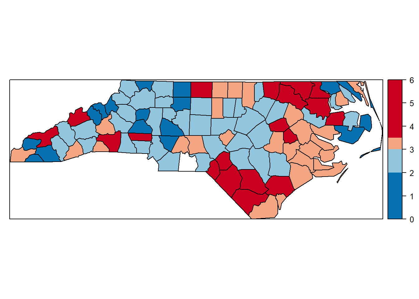
##Compute Moran's I and Geary's C
nc.sids.moran.out = moran.test(nc.sids.rates.FT, listw=ncCC89.listw, zero.policy=TRUE)
nc.sids.geary.out = geary.test(nc.sids.rates.FT, listw=ncCC89.listw, zero.policy=TRUE)

nc.sids.moran.out
##
## Moran I test under randomisation
##
## data: nc.sids.rates.FT
## weights: ncCC89.listw n reduced by no-neighbour observations
##
##
## Moran I statistic standard deviate = 3.8188, p-value = 6.704e-05
## alternative hypothesis: greater
## sample estimates:
## Moran I statistic Expectation Variance
## 0.253677291 -0.010309278 0.004778579nc.sids.geary.out##
## Geary C test under randomisation
##
## data: nc.sids.rates.FT
## weights: ncCC89.listw
##
## Geary C statistic standard deviate = 3.3996, p-value = 0.0003374
## alternative hypothesis: Expectation greater than statistic
## sample estimates:
## Geary C statistic Expectation Variance
## 0.694318792 1.000000000 0.008084976We wish to regress these rates on the non-white birth rates over the same period. Let \(x_i\) be the Freeman-Tukey transformation of non-white birth rate in county \(i\). Here is the model. \[w_i = \beta_0 + \beta_1 x_i + u_i,\] where \(u_i, i = 1,2,...,n\) are modeled by Gaussian CAR model with parameters \(\tau^2\) and \(\rho\). We also compare the above model with non-spatial regression model and pure CAR model without predictors.
##Begin with a Freeman-Tukey transformation on non-white birth rates
nc.sids.nwbir.FT = sqrt(1000) * (sqrt(nc.sids$NWBIR74/nc.sids$BIR74)
                                 + sqrt((nc.sids$NWBIR74 + 1)/nc.sids$BIR74))
nc.sids$nwbir.FT = nc.sids.nwbir.FT

#non-spatial regression of z_i on x_i.
plot(nc.sids$nwbir.FT, nc.sids$rates.FT)
abline(lsfit(nc.sids$nwbir.FT, nc.sids$rates.FT),lty=2,col=1)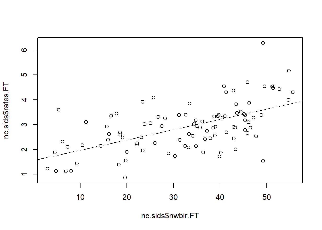
m1 <- lm(nc.sids$rates.FT~nc.sids$nwbir.FT)
nc.sids$fitted.nonsp.reg <- m1$fitted.values
summary(m1)
##
## Call:
## lm(formula = nc.sids$rates.FT ~ nc.sids$nwbir.FT)
##
## Residuals:
## Min 1Q Median 3Q Max
## -2.05032 -0.57392 0.01278 0.46939 2.68873
##
## Coefficients:
## Estimate Std. Error t value Pr(>|t|)
## (Intercept) 1.555085 0.205045 7.584 1.94e-11 ***
## nc.sids$nwbir.FT 0.041401 0.005794 7.146 1.60e-10 ***
## ---
## Signif. codes: 0 '***' 0.001 '**' 0.01 '*' 0.05 '.' 0.1 ' ' 1
##
## Residual standard error: 0.7954 on 98 degrees of freedom
## Multiple R-squared: 0.3426, Adjusted R-squared: 0.3358
## F-statistic: 51.06 on 1 and 98 DF, p-value: 1.603e-10nc.sids.res.moran.out = moran.test(m1$residuals, listw=ncCC89.listw, zero.policy=TRUE)
nc.sids.res.moran.out##
## Moran I test under randomisation
##
## data: m1$residuals
## weights: ncCC89.listw n reduced by no-neighbour observations
##
##
## Moran I statistic standard deviate = 0.78707, p-value = 0.2156
## alternative hypothesis: greater
## sample estimates:
## Moran I statistic Expectation Variance
## 0.044091695 -0.010309278 0.004777374##CAR model regressing z_i on x_i
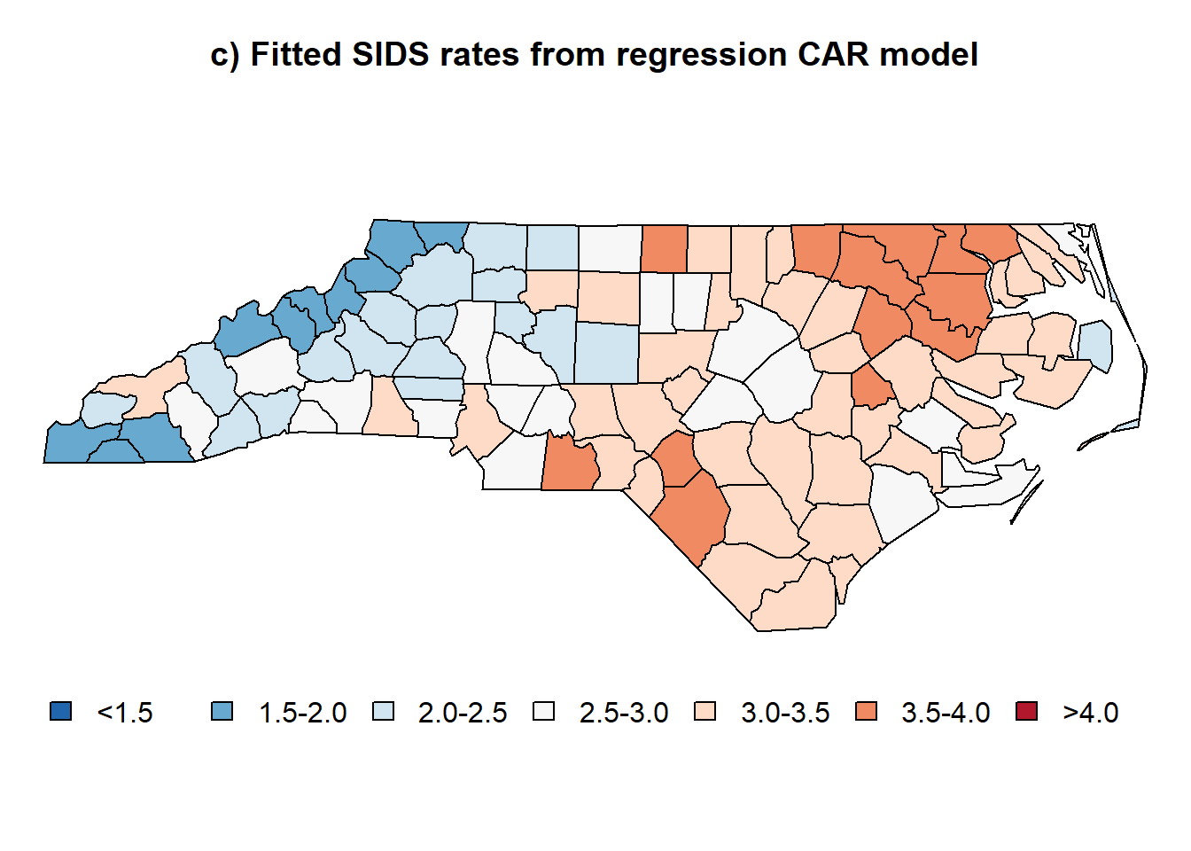
nc.sids.car.out = spautolm(rates.FT~ nwbir.FT, data=nc.sids, family="CAR",
listw=ncCC89.listw, zero.policy=TRUE)
nc.sids.car.fitted = fitted(nc.sids.car.out)
nc.sids$fitted.car = nc.sids.car.fitted
summary(nc.sids.car.out)##
## Call:
## spautolm(formula = rates.FT ~ nwbir.FT, data = nc.sids, listw = ncCC89.listw,
## family = "CAR", zero.policy = TRUE)
##
## Residuals:
## Min 1Q Median 3Q Max
## -2.0774294 -0.5528606 0.0063236 0.4856087 2.7074144
##
## Regions with no neighbours included:
## 37055 37095
##
## Coefficients:
## Estimate Std. Error z value Pr(>|z|)
## (Intercept) 1.5440567 0.2187047 7.060 1.665e-12
## nwbir.FT 0.0419258 0.0061466 6.821 9.043e-12
##
## Lambda: 0.043228 LR test value: 0.39416 p-value: 0.53012
## Numerical Hessian standard error of lambda: 0.06653
##
## Log likelihood: -117.8018
## ML residual variance (sigma squared): 0.61526, (sigma: 0.78438)
## Number of observations: 100
## Number of parameters estimated: 4
## AIC: 243.6#pure CAR model without regression
nc.sids.pure.car.out = spautolm(rates.FT~ 1, data=nc.sids, family="CAR",
listw=ncCC89.listw, zero.policy=TRUE)
nc.sids.pure.car.fitted = fitted(nc.sids.pure.car.out)
nc.sids$fitted.pure.car = nc.sids.pure.car.fitted
summary(nc.sids.pure.car.out)##
## Call: spautolm(formula = rates.FT ~ 1, data = nc.sids, listw = ncCC89.listw,
## family = "CAR", zero.policy = TRUE)
##
## Residuals:
## Min 1Q Median 3Q Max
## -1.726462 -0.538181 -0.021378 0.475053 3.434710
##
## Regions with no neighbours included:
## 37055 37095
##
## Coefficients:
## Estimate Std. Error z value Pr(>|z|)
## (Intercept) 2.98093 0.14292 20.858 < 2.2e-16
##
## Lambda: 0.15546 LR test value: 10.667 p-value: 0.0010909
## Numerical Hessian standard error of lambda: 0.028893
##
## Log likelihood: -133.6352
## ML residual variance (sigma squared): 0.79142, (sigma: 0.88962)
## Number of observations: 100
## Number of parameters estimated: 3
## AIC: 273.27#Draw the maps using the maps function
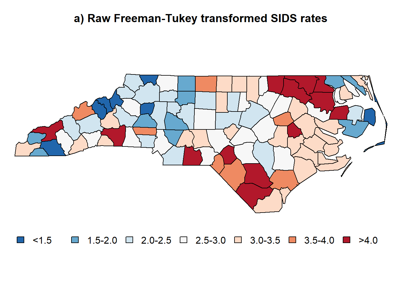
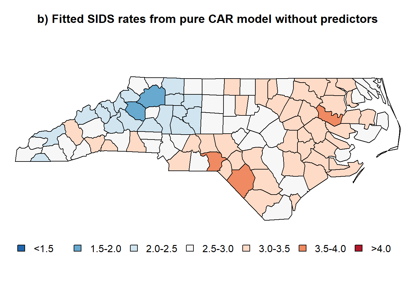
brks = c(0, 1.5, 2.0, 2.5, 3.0, 3.5, 4.0, 6.5)
nCol = length(brks) -1
color.pallete = rev(brewer.pal(nCol,"RdBu"))
class.raw = classIntervals(var=nc.sids$rates.FT, n=nCol, style="fixed",
fixedBreaks=brks, dataPrecision=nCol)
color.code.raw = findColours(class.raw, color.pallete)
class.fitted.pure.car = classIntervals(var=nc.sids$fitted.pure.car, n=nCol,
style="fixed", fixedBreaks=brks, dataPrecision=nCol)
color.code.fitted.pure.car = findColours(class.fitted.pure.car, color.pallete)
class.fitted.car = classIntervals(var=nc.sids$fitted.car, n=nCol, style="fixed",
fixedBreaks=brks, dataPrecision=nCol)
color.code.fitted.car = findColours(class.fitted.car, color.pallete)
class.fitted.nonsp.reg = classIntervals(var=nc.sids$fitted.nonsp.reg, n=nCol,
style="fixed", fixedBreaks=brks, dataPrecision=nCol)
color.code.fitted.nonsp.reg = findColours(class.fitted.nonsp.reg, color.pallete)
leg.txt = c("<1.5", "1.5-2.0", "2.0-2.5", "2.5-3.0", "3.0-3.5", "3.5-4.0", ">4.0")
if(1){
par(mar=c(3.1,0,3.1,0))
plot(nc.sids, col=color.code.raw);
title("a) Raw Freeman-Tukey transformed SIDS rates", cex = 0.5 )
legend("bottom", legend=leg.txt, cex=1, bty="n", horiz = TRUE, fill = color.pallete)
plot(nc.sids, col=color.code.fitted.pure.car)
title("b) Fitted SIDS rates from pure CAR model without predictors", cex = 0.5 )
legend("bottom", legend=leg.txt, cex=1, bty="n", horiz = TRUE, fill = color.pallete)
plot(nc.sids, col=color.code.fitted.car)
title("c) Fitted SIDS rates from regression CAR model", cex = 0.5)
legend("bottom", legend=leg.txt, cex=1, bty="n", horiz = TRUE, fill = color.pallete)
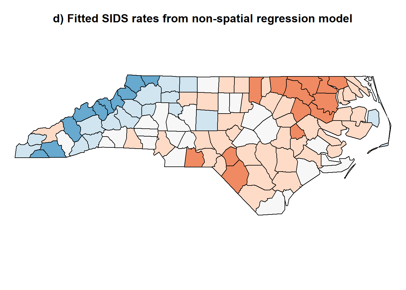
plot(nc.sids, col=color.code.fitted.nonsp.reg)
title("d) Fitted SIDS rates from non-spatial regression model", cex = 0.5)
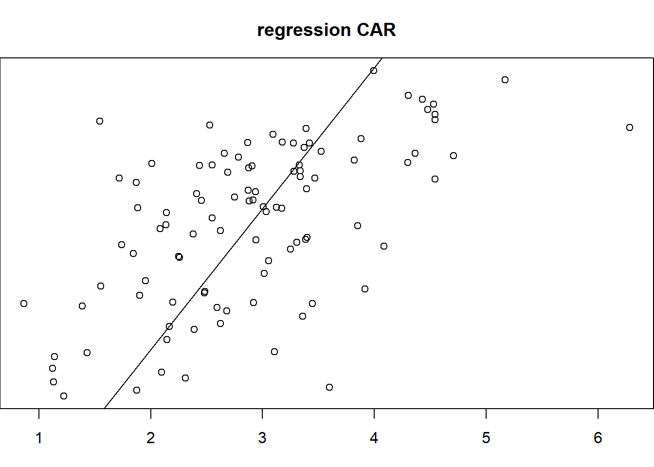
plot(nc.sids$rates.FT,nc.sids$fitted.car, ylab = "fitted", xlab = "obs",
main = "regression CAR")
abline(a = 0, b = 1)
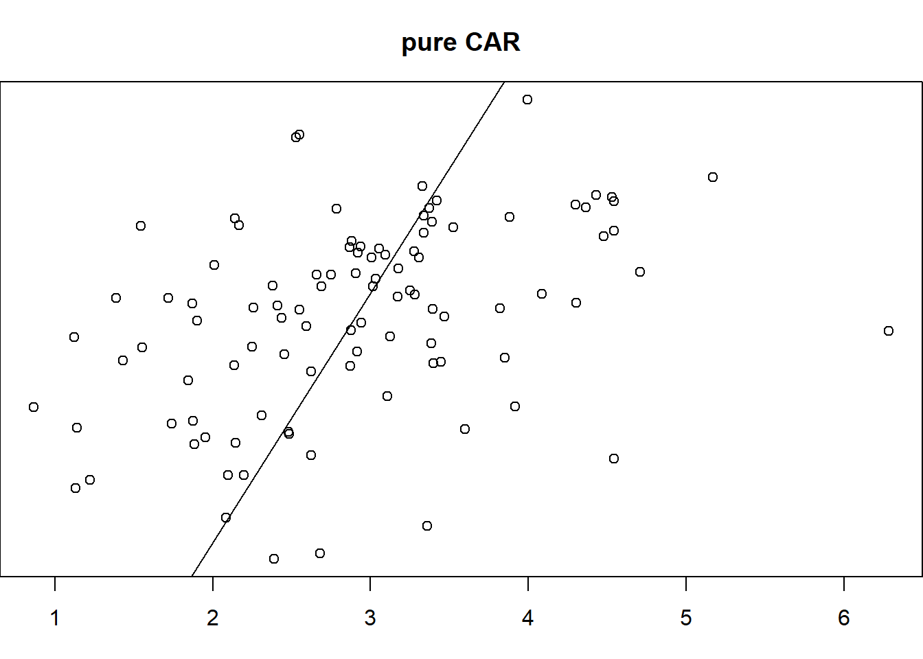
plot(nc.sids$rates.FT,nc.sids$fitted.pure.car, ylab = "fitted", xlab = "obs",
main = "pure CAR")
abline(a = 0, b = 1)
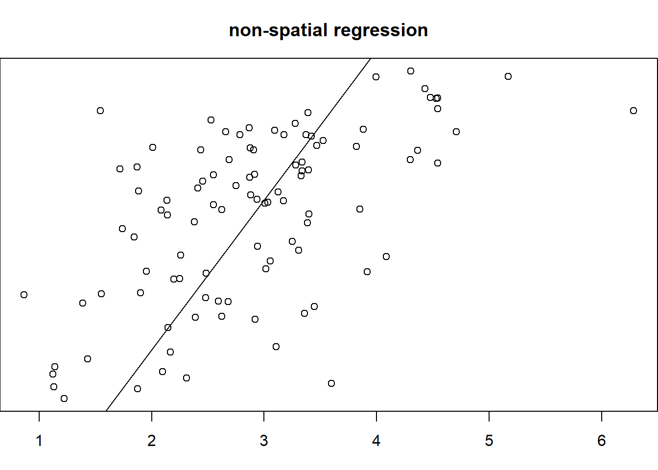
plot(nc.sids$rates.FT, nc.sids$fitted.nonsp.reg, ylab = "fitted", xlab = "obs",
main = "non-spatial regression")
abline(a = 0, b = 1)
}
For the non-Gaussian CAR model, a typical model would be auto logistic CAR model introduced in Example 4.4. We’ll not go details in this class.
4.3 Applications: Disease mapping
An area of strong biostatistical and epidemiological interest is that of disease mapping. The aim of disease mapping is to provide a representation of the spatial distribution of the risk of a disease in the study area, which consists of several non-overlapping smaller regions. The risk may reflect actual deaths due to the disease (mortality), or, if it is not fatal, the number of people who suffer from the disease (morbidity) in a certain period of time for the population at risk.
To begin, suppose we observe counts of cases of disease \(Y_i\) in region \(i\), \(i=1,2,...,I\). \(Y_i\)s are considered as random variables. Other data include either the local number of individuals at risk \(n_i\) or the expected number of disease cases \(E_i\) in region \(i\), \(i=1,2,...,I\). \(E_i\) are considered as fixed and known functions of \(n_i\). As a simple starting point, we assume that \[E_i = n_i r,\] where \(r = \sum_i Y_i/(\sum_i n_i)\) is the overall disease rate in the entire study region. These \(E_i\) are defined under the assumption of constant risk for all individuals. It can be generalized to fit more realistic situations. For example, if the disease rates vary with ages, then we could get the overall disease rates for people within each age group, say \(r_{1}, ..., r_{J}\), where \(J\) is the number of groups classified by ages, and the expected disease cases in region \(i\) is given by \[E_i = \sum_j n_{ij} r_{j},\] where \(n_{ij}\) is the number of individuals at risk in region \(i\) who belong to age group \(j\).
4.3.1 Traditional models and freqentist methods
When \(E_i\) is not large (i.e., the disease rate or the region \(i\) are sufficiently small), the usual model for \(Y_i\) is the Poisson model,
\[Y_i \,|\, \eta_i \sim Poisson(E_i \eta_i),\] where \(\eta_i\) is the true relative risk of disease in region \(i\). The MLE of \(\eta_i\) is easily derived, \[\hat \eta_i = \frac{Y_i}{E_i},\] which is so called standardized morbidity (or mortality) ratio (SMR), that is, the ratio of observed to expected disease cases (or deaths). Further, we can see the variance of SMR is \[\text{Var}(\hat \eta_i) = \eta_i /E_i.\] Suppose we wish to test whether the true relative risk in region \(i\) is elevated or not, that is, \[H_0: \eta_i = 1,\ vs. \ H_a: \eta_i >1.\] Under null hypothesis, \(Y_i\sim Poisson(E_i)\), so the p-value of the test is \[\text{p value} = 1- \sum_{k=0}^{Y_i-1}\frac{E_i^ke^{-E_i}}{k!}.\] If p value is small (i.e., less than 0.05), we reject \(H_0\) and conclude that there is a statistically significant excess risk in region \(i\).
4.3.2 Hierarchical Bayesian methods
In order to borrow information across regions, here we introduce a hierarchical Bayesian spatial model. Suppose \((X_{i1},...,X_{ip})^\top\) are explanatory variables in region \(i\) and let \({\mathbf{X}}_i = (1, X_{i1},...,X_{ip})^\top\) which includes the intercept. We model \(\log(\eta_i)\) by a spatial IAR model.
Recall that \(W\) is a symmetric proximity (spatial neighborhood) matrix of regions \(1,2,...,I\). \(w_{ij}\) is set to zero if site \(i\) and \(j\) are neighbors; otherwise, \(w_{ij}=0\). Let the \(i\)th row sum of the matrix \(W\) be \(w_{i+} = \sum_{j=1}^n w_{ij}\).
\[ \begin{align*} &Y_i \,|\, v_i \stackrel{ind.}{\sim} Poisson(E_i \eta_i)\\ &log(\eta_i) = {\mathbf{X}}_i^\top {\boldsymbol{\beta}}+v_i\\ & v_i \,|\, v_{-i} \sim Gaussian(\sum_{j} w_{ij}v_{j}/w_{i+}, \tau^2/w_{i+}), i = 1,2,...,I\\ & p({\boldsymbol{\beta}}, \tau^2) \sim Gaussian(\textbf{0}, \sigma_\beta^2)\times IG(a_{\tau^2}, b_{\tau^2}). \end{align*} \]
As we know, the joint density of intrinsically autoregressive (IAR) random vector \((v_1,...,v_i)\) is improper. Here we use it to model the random effect rather than the data. The posterior distribution of the data can still be proper. But it also requires some care because the IAR model can only identify the pairwise difference \(v_i-v_j\), but not identify the overall mean of \(v_1,...,v_I\). Thus to identify an intercept term \(\beta_0\) in the log relative risk \(\log(\eta_i)\), we must add the constraint \(\sum_{i=1}^I v_i = 0\). This additional constraint slightly complicates the implementation of MCMC algorithm, that is, replacing \(v_i\) with \(v_i - \bar v\) in each MCMC iteration, where \(\bar v\) is the average of \(v_i\)s.
In the above model, \(v_i\)s capture regional clustering. That is, they model extra-Poisson variability in the log-relative risks that varies “locally”, so that nearby regions will have more similar rates. A further extension of the above model is to incorporate an additional random effect \(u_i\) (see, e.g., Besag, York, and Mollié (1991)), which capture extra-Poisson variability in the log-relative risk that varies “globally”, i.e., over the entire study region. Specifically, the model is given by
\[ \begin{align*} &Y_i \,|\, v_i, u_i \stackrel{ind.}{\sim} Poisson(E_i \eta_i)\\ &log(\eta_i) = {\mathbf{X}}_i^\top {\boldsymbol{\beta}}+v_i + u_i\\ & v_i \,|\, v_{-i} \sim Gaussian(\sum_{j} w_{ij}v_{j}/w_{i+}, \tau_v^2/w_{i+})\\ & u_i \stackrel{ind.}{\sim} Gaussian(0, \tau_u^2), i = 1,2,...,I\\\\ & p({\boldsymbol{\beta}}, \tau_v^2, \tau_u^2) \sim Gaussian(\textbf{0}, \sigma_\beta^2)\times IG(a_{\tau_v^2}, b_{\tau_v^2})\times IG(a_{\tau_u^2}, b_{\tau_u^2}). \end{align*} \] We end this section by applying the above methods to SIDS data (see, e.g., Bivand et al. (2008)).
#disease mapping
rm(list=ls())
#read in sids data
library(maptools)
library(spdep)
nc_file <- system.file("shapes/sids.shp", package="spData")[1]
llCRS <- CRS("+proj=longlat +datum=NAD27")
nc <- readShapePoly(nc_file, ID="FIPSNO", proj4string=llCRS)
rn <- sapply(slot(nc, "polygons"), function(x) slot(x, "ID"))
gal_file <- system.file("weights/ncCR85.gal", package="spData")[1]
ncCR85 <- read.gal(gal_file, region.id = rn)

#Yi
nc$Observed <- nc$SID74
#ni
nc$Population <- nc$BIR74
r <- sum(nc$Observed)/sum(nc$Population)
#Ei
nc$Expected <- nc$Population*r
#SMR
nc$SMR <- nc$Observed/nc$Expected

#plot of SMR
library(RColorBrewer)
logSMR <- log(nc$SMR[nc$SMR>0])
nsteps <- 7
step <- (max(logSMR)-min(logSMR))/nsteps
brks <- exp(min(logSMR)+(0:nsteps)*step)
brks[1] <- 0
cols <- c(rev(brewer.pal(3, "Blues")), brewer.pal(4, "Reds"))
grps <- as.ordered(cut(nc$SMR, brks, include.lowest=TRUE))
plot(nc, col=cols[unclass(grps)], axes = FALSE)
box()
degAxis(1)
degAxis(2)
legend("bottomleft",legend=levels(grps), fill=cols, bty="n",cex=0.8,y.intersp=0.8)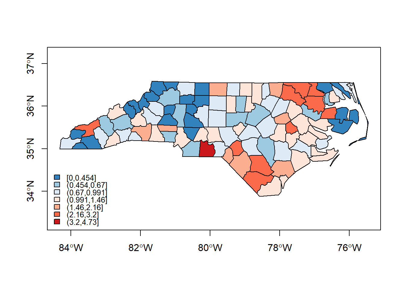
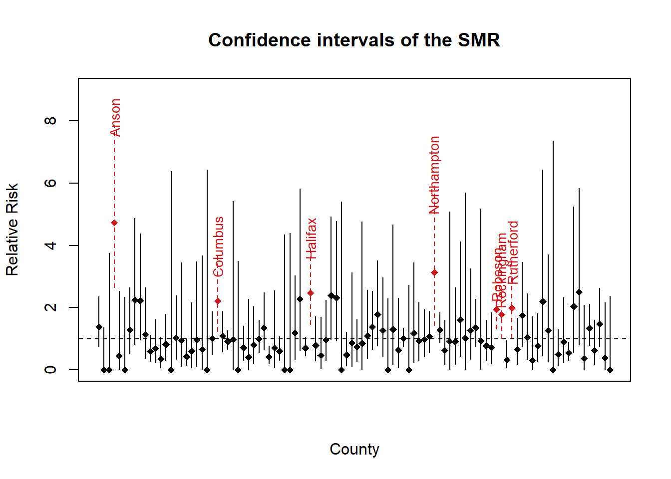
#CIs of SMR
library(epitools)
CISMR <- pois.exact(nc$Observed, nc$Expected)
plot(1,1, type="n", xlim=c(1,100), ylim=c(0,9),
     main= "Confidence intervals of the SMR",
     xlab="County", ylab="Relative Risk", xaxt="n")
abline(h=1, lty=2)

for(i in 1:100) {
  if(CISMR$lower[i]>1 ) {
    sig.col <- brewer.pal(4, "Reds")[4]
    col <- sig.col
    lty <- 2
    text(i, CISMR$upper[i]+.31, nc$NAME[i],
         srt=90, col=sig.col, cex=.85)
  } else {
    col <- "black"
    lty <- 1
  }
  lines(c(i,i), c(CISMR$lower[i],CISMR$upper[i]), col=col, lty=lty)
  points(i, nc$SMR[i], pch=18, col=col)
}
#BYM model (Besag et al. (1991)).
#WinBUGS is a free software that uses MCMC methods, in particular, Gibbs sampling.
#It can be downloaded from https://www.mrc-bsu.cam.ac.uk/software/bugs/the-bugs-project-winbugs/
#"R2WinBUGS" is a package for using WinBUGS from R.
library(R2WinBUGS)
#proximity matrix
nc.nb <- nb2WB(ncCR85)

#calculate the non-white birth proportion and consider it as an explanatory variable for
#the log relative risk
nc$nwprop <- nc$NWBIR74/nc$BIR74

#"d": data object in R with non-white birth proportion
N <- length(nc$Observed)
d <- list(N=N, observed=nc$Observed, expected=nc$Expected,
          nonwhite=nc$nwprop,
          adj=nc.nb$adj,  weights=nc.nb$weights, num=nc.nb$num)

#"dwoutcov": data object in R without predictors
dwoutcov <- list(N=N, observed=nc$Observed, expected=nc$Expected,
                 adj=nc.nb$adj,  weights=nc.nb$weights, num=nc.nb$num)

#initial value of parameters, precu: 1/tau_u^2, precv: 1/tau_v^2
inits <- list(u=rep(0,N), v=rep(0,N), alpha=0, beta=0, precu=.001, precv=.001)

#the WinBUGS codes for implementing BYM model is saved in "BYM-model.txt"
bymmodelfile <- paste(getwd(), "/BYM-model.txt", sep="")
#wdir: the working directory
wdir <- paste(getwd(), "/BYM", sep="")
if(!file.exists(wdir)){dir.create(wdir)}
#BugsDir: the directory where the software "WinBUGS14" is saved
BugsDir <- "C:/WinBUGS14"

#The function "bugs" takes as input data, initial values, model file and other info required,
#and creates a script that will be run with WinBUGS. The output files are saved in "wdir".
MCMCres<- bugs(data = d, inits = list(inits),
  working.directory = wdir,
  parameters.to.save = c("theta", "alpha", "beta", "u", "v", "sigmau", "sigmav"),
  n.chains = 1, n.iter = 30000, n.burnin = 20000, n.thin = 10,
  model.file = bymmodelfile,
  bugs.directory = BugsDir)

#save posterior mean of eta_i, u_i and v_i to nc.
nc$BYM.eta.mean <- MCMCres$mean$theta
nc$BYM.u.mean <- MCMCres$mean$u
nc$BYM.v.mean <- MCMCres$mean$v

#the output files "coda1.txt" and "codaIndex.txt" contain the simulations from all the variables
#saved in WinBUGS
library(coda)
nc.output <- read.coda("BYM/coda1.txt", "BYM/codaIndex.txt", quiet = TRUE)
plot(nc.output[,c("deviance")])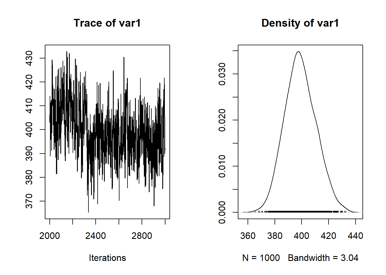
plot(nc.output[,c("alpha")])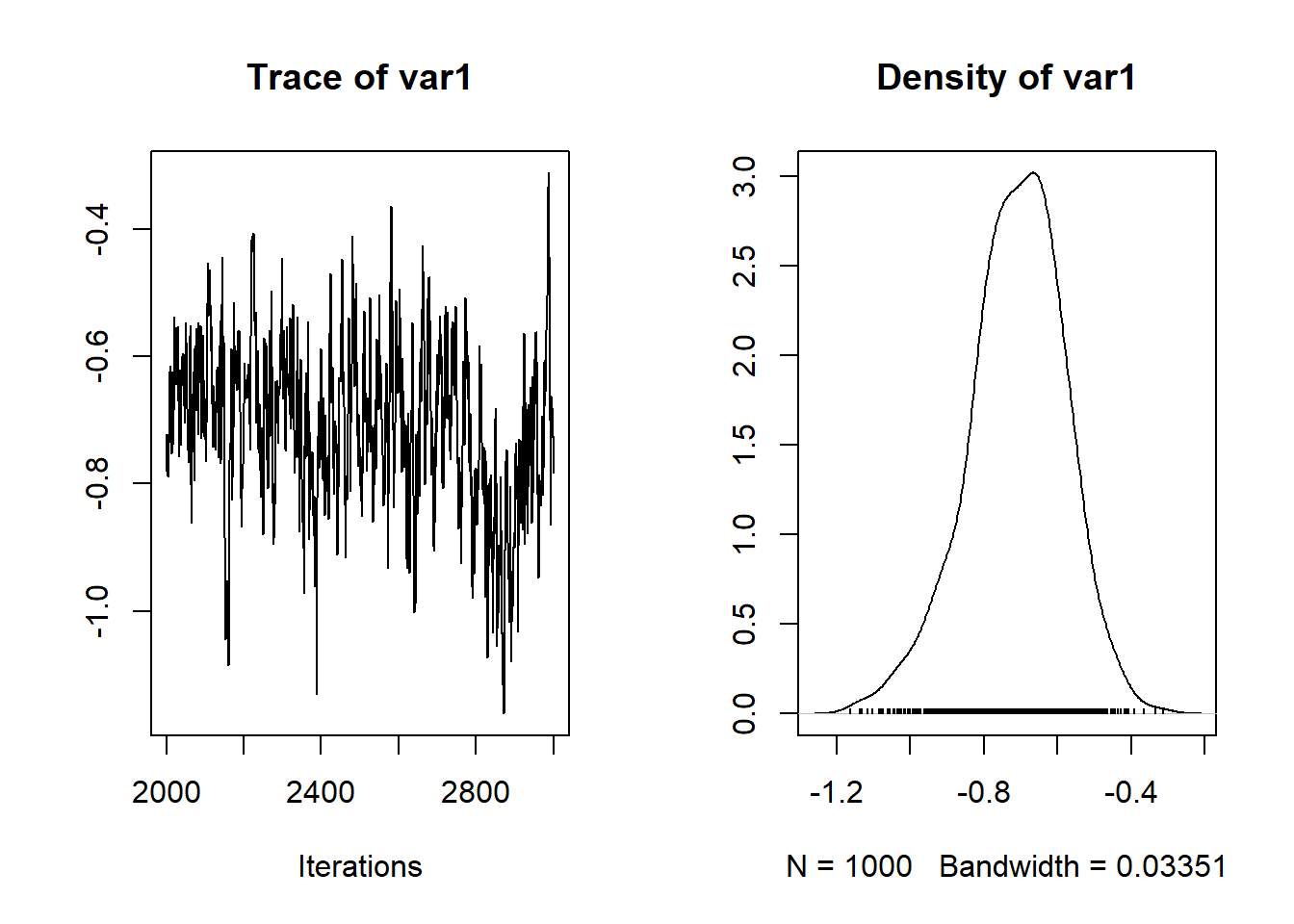
plot(nc.output[,c("beta")])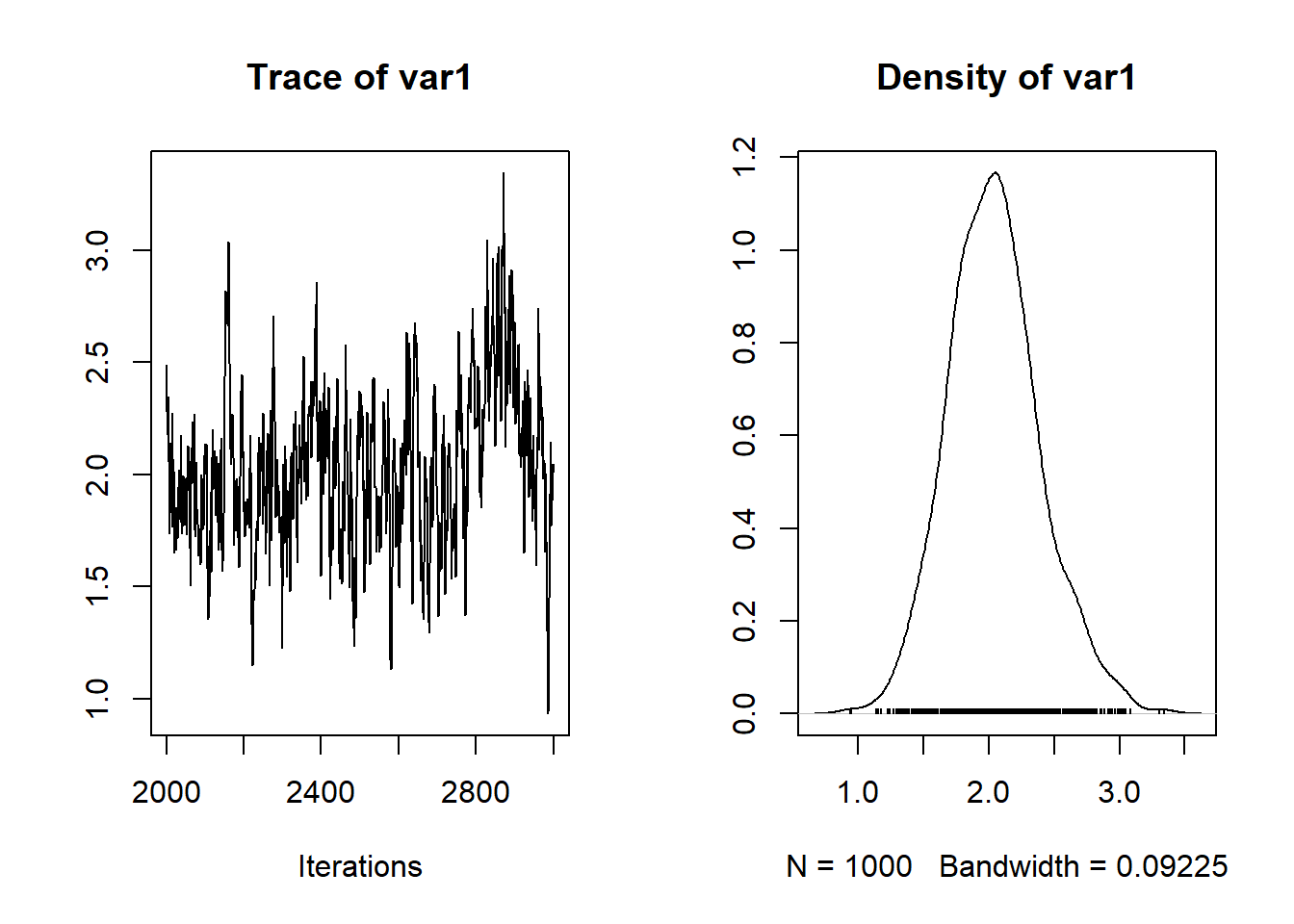
#MCMC chain of the relative risk of Robeson county (area number 94)
plot(nc.output[,c("theta[94]")])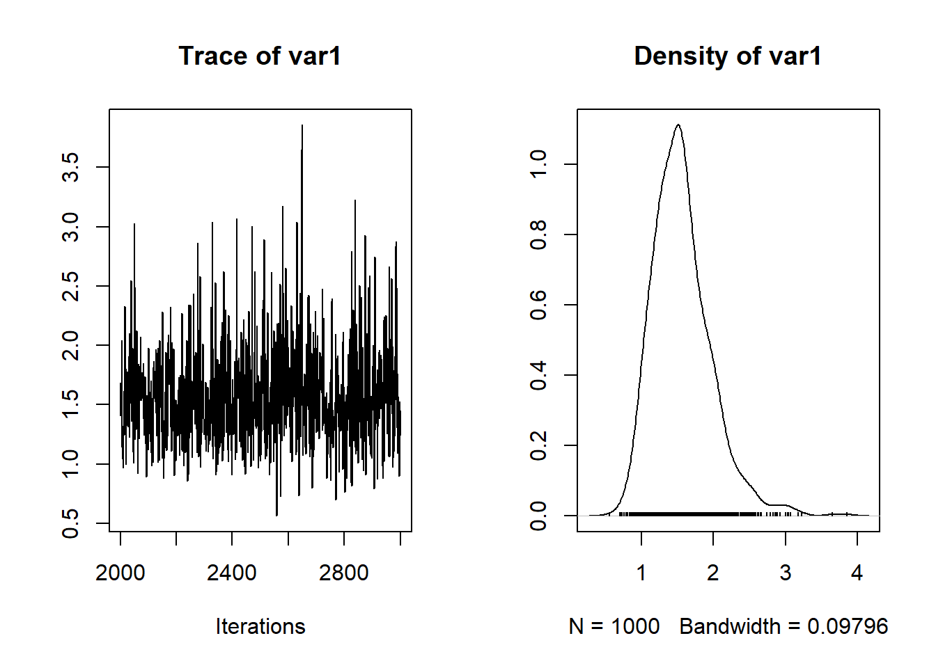
#compare the raw SMR and the posterior mean of SMR
spplot(nc, c("SMR", "BYM.eta.mean"), at=brks, col.regions=cols, axes=TRUE)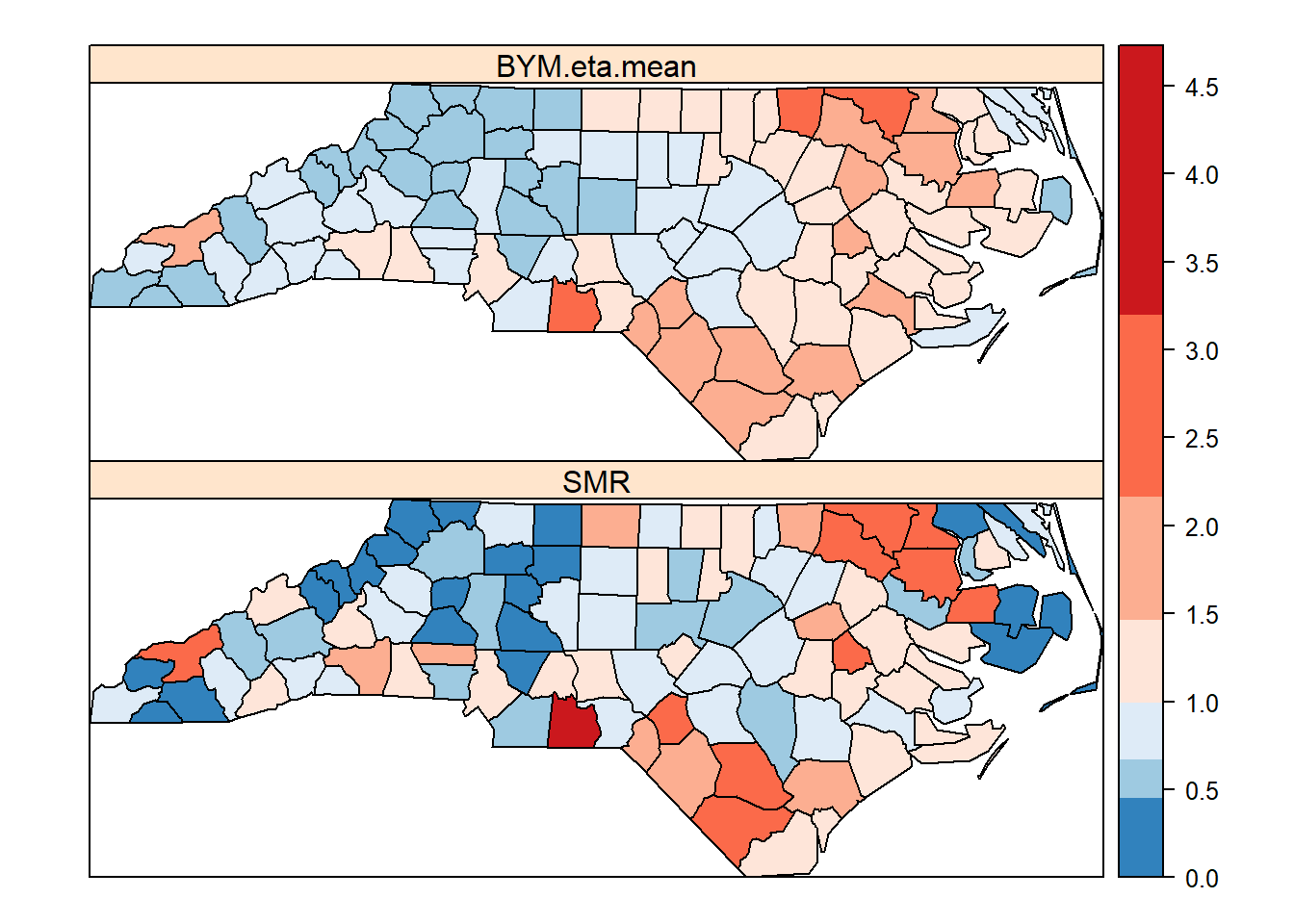
#posterior mean of random effect u and v
ubrks <- quantile(nc$BYM.u.mean, seq(0,1,1/5))
ubrks[6] <- ubrks[6]*1.01
#RSB
ubrks <- seq(-0.35, 0.35, 0.05)
spplot(nc, c("BYM.u.mean", "BYM.v.mean"), at= ubrks, axes=TRUE,
             col.regions=c(rev(brewer.pal(7, "Reds")), brewer.pal(7, "Blues")))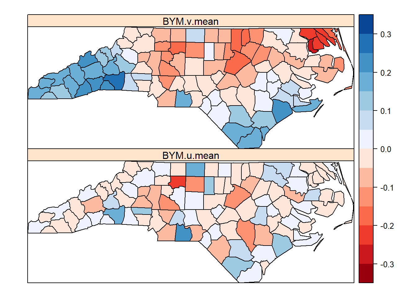
#95% posterior CIs for SMR under BYM model
plot(1,1, type="n", xlim=c(1,100), ylim=c(0,5),
     main= "95% posterior intervals of the relative risks",
     xlab="County", ylab="Relative Risk", xaxt="n")
abline(h=1, lty=2)

for(i in 1:100)
{
  if(MCMCres$summary[i,3]>1 )
  {
    #col <- gray(.4)
    col <- sig.col
    lty <- 2
    text(i, MCMCres$summary[i,7]+.31, nc$NAME[i],
         srt=90, col=sig.col, cex=.85)
  }
  else
  {
    col <- "black"
    lty <- 1
  }

  lines(c(i,i), c(MCMCres$summary[i,3], MCMCres$summary[i,7]), col=col, lty=lty)
}

points(1:100, MCMCres$median$theta, pch=18, col=col)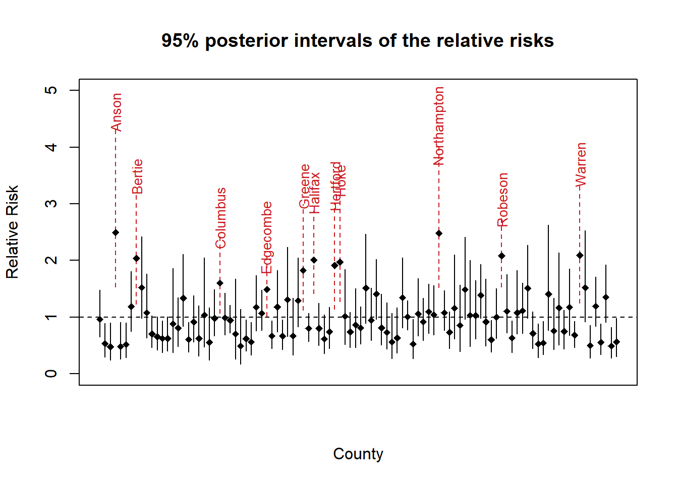
References
Besag, Julian. 1974. “Spatial Interaction and the Statistical Analysis of Lattice Systems.” Journal of the Royal Statistical Society. Series B (Methodological). JSTOR, 192–236.
Besag, Julian, Jeremy York, and Annie Mollié. 1991. “Bayesian Image Restoration, with Two Applications in Spatial Statistics.” Annals of the Institute of Statistical Mathematics 43 (1): 1–20. doi:10.1007/BF00116466.
Bivand, Roger S, Edzer J Pebesma, Virgilio Gómez-Rubio, and Edzer Jan Pebesma. 2008. Applied Spatial Data Analysis with R. Vol. 747248717. Springer.
Cressie, N.A.C. 1993. Statistics for spatial data, 2nd ed. New York: Jone Wiley & Sons.