Chapter 3 Geostatistical data analysis (Continuous spatial variation)

In this chapter, we’ll focus on statistical analysis for geostatistical data, including estimation, inference and predictions.

N. Cressie (1993) suggested the following modeling framework for geostatistical data. For any \({\mathbf{s}}\in \mathcal{D}\), \[Y({\mathbf{s}}) = \mu ({\mathbf{s}}) + w({\mathbf{s}}) + \eta({\mathbf{s}}) + \epsilon({\mathbf{s}}),\] where

i). The mean function \(\mu({\mathbf{s}})\) is the large scale trend of the random field. If there are other predictors, say \({\mathbf{X}}({\mathbf{s}}) = (X_1({\mathbf{s}}), ..., X_p({\mathbf{s}}))^\top\), then \(\mu({\mathbf{s}})\) in general can be considered as a function of \({\mathbf{s}}\) and \({\mathbf{X}}({\mathbf{s}})\);

ii). \(w({\mathbf{s}})\) is a random field with mean zero, which models the smooth-scale variation. Usually it is modeled by a weakly stationary random field with covariance function \(C_w({\mathbf{h}})\);

iii). \(\eta({\mathbf{s}})\) is another random field with mean zero, which models the micro-scale variation. It is used to describe the spatial variability within the range \(r\leq \min_{i,j}\{||{\mathbf{s}}_i-{\mathbf{s}}_j||\}\). So it cannot be estimated from the observed data. We may only be able to estimate \({\text{Var}}(\eta({\mathbf{s}})) = \sigma^2_\eta\);

iv). \(\epsilon({\mathbf{s}})\) denotes the white noise measurement error with variance \(\sigma_\epsilon^2\). Indeed, \(\{\epsilon({\mathbf{s}}), {\mathbf{s}}\in \mathcal{D}\}\) are a collection of independent random variables with mean zero and variance \(\sigma_\epsilon^2\);

v). \(w({\mathbf{s}})\), \(\eta({\mathbf{s}})\) and \(\epsilon({\mathbf{s}})\) are independent with each other.

However, unless there are replications in the data, \(\sigma_\eta^2\) and \(\sigma_\epsilon^2\) cannot be estimated separately. In application, most of time we ignore the spatial dependence of \(\eta({\mathbf{s}})\) but merge its marginal variance \(\sigma^2_\eta\) to \(\epsilon({\mathbf{s}})\). Hence, we ends up a spatial model as following,

\[Y({\mathbf{s}}) = \mu ({\mathbf{s}}) + w({\mathbf{s}}) + e({\mathbf{s}}),\] where \(e({\mathbf{s}})\) denotes white noise with variance \(\sigma_e^2=\sigma_\eta^2+\sigma_\epsilon^2\).

The last thing we have to specify is how to model the covariance function of \(w({\mathbf{s}})\). Usually, we’ll use a parametric positive definite function to model \(C_w({\mathbf{h}})\).

3.1 Covariance models and semivariogram models

In this section, we introduce several most popular covariance functions and provide the definition of semivariogram.

3.1.1 Matérn covariance function

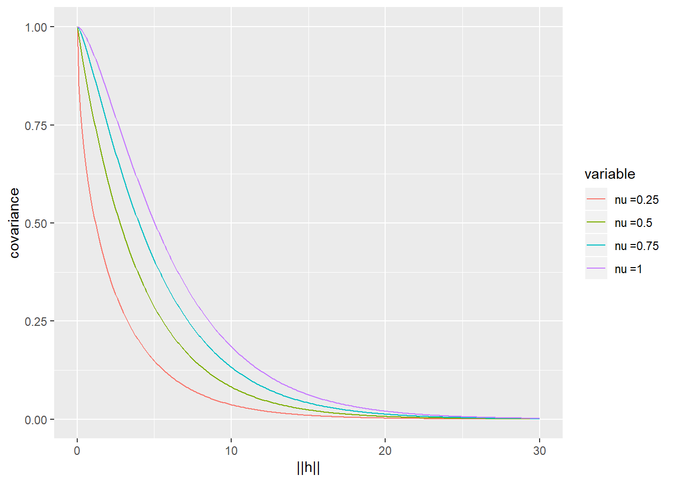
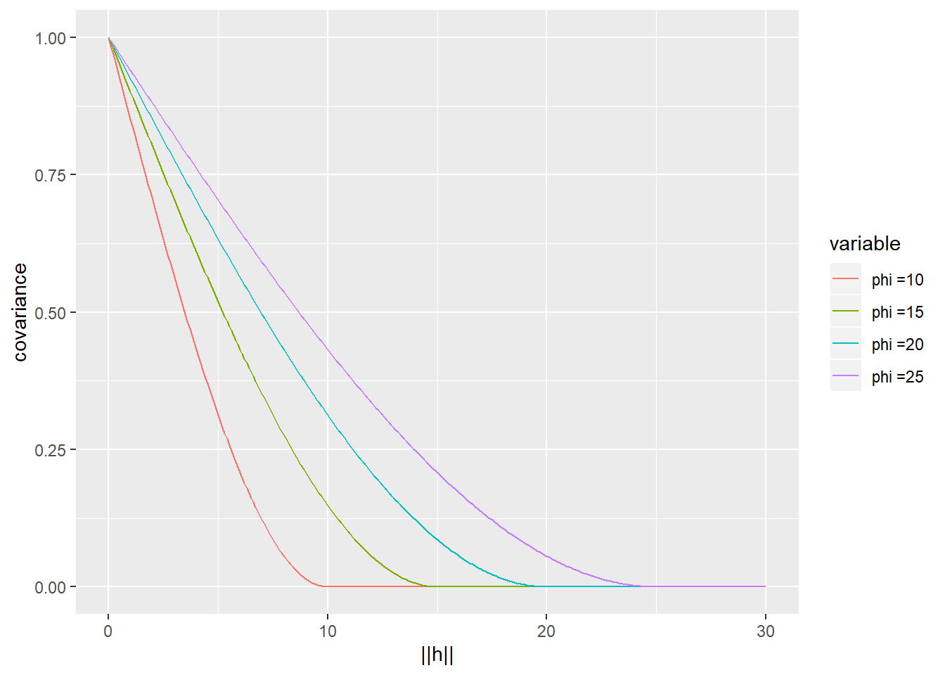
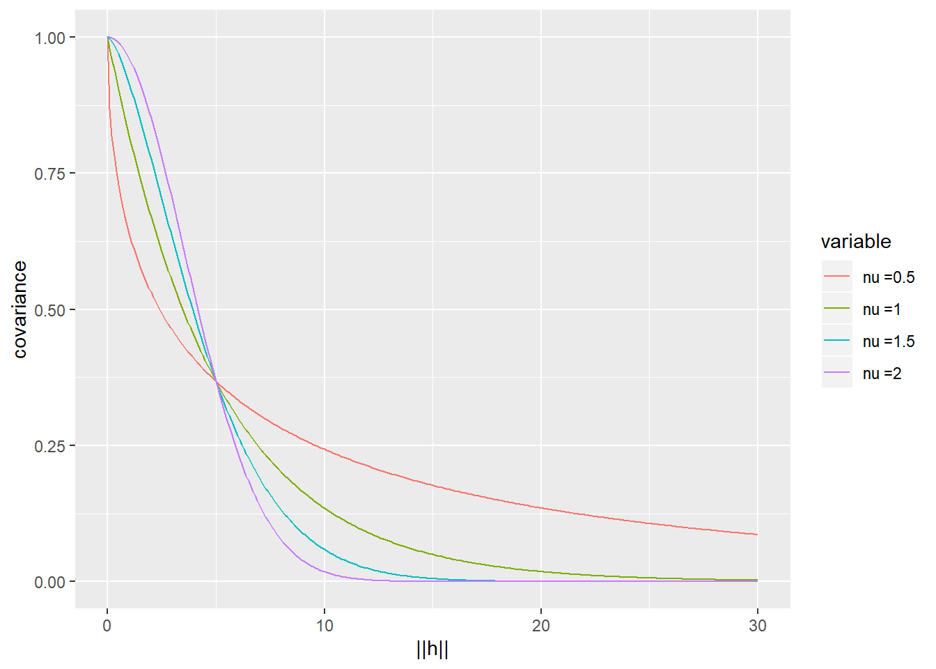
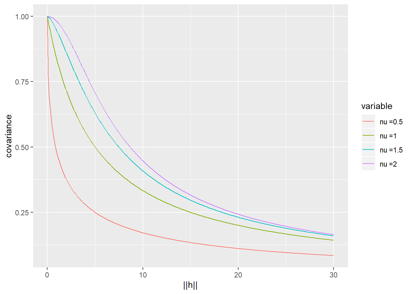
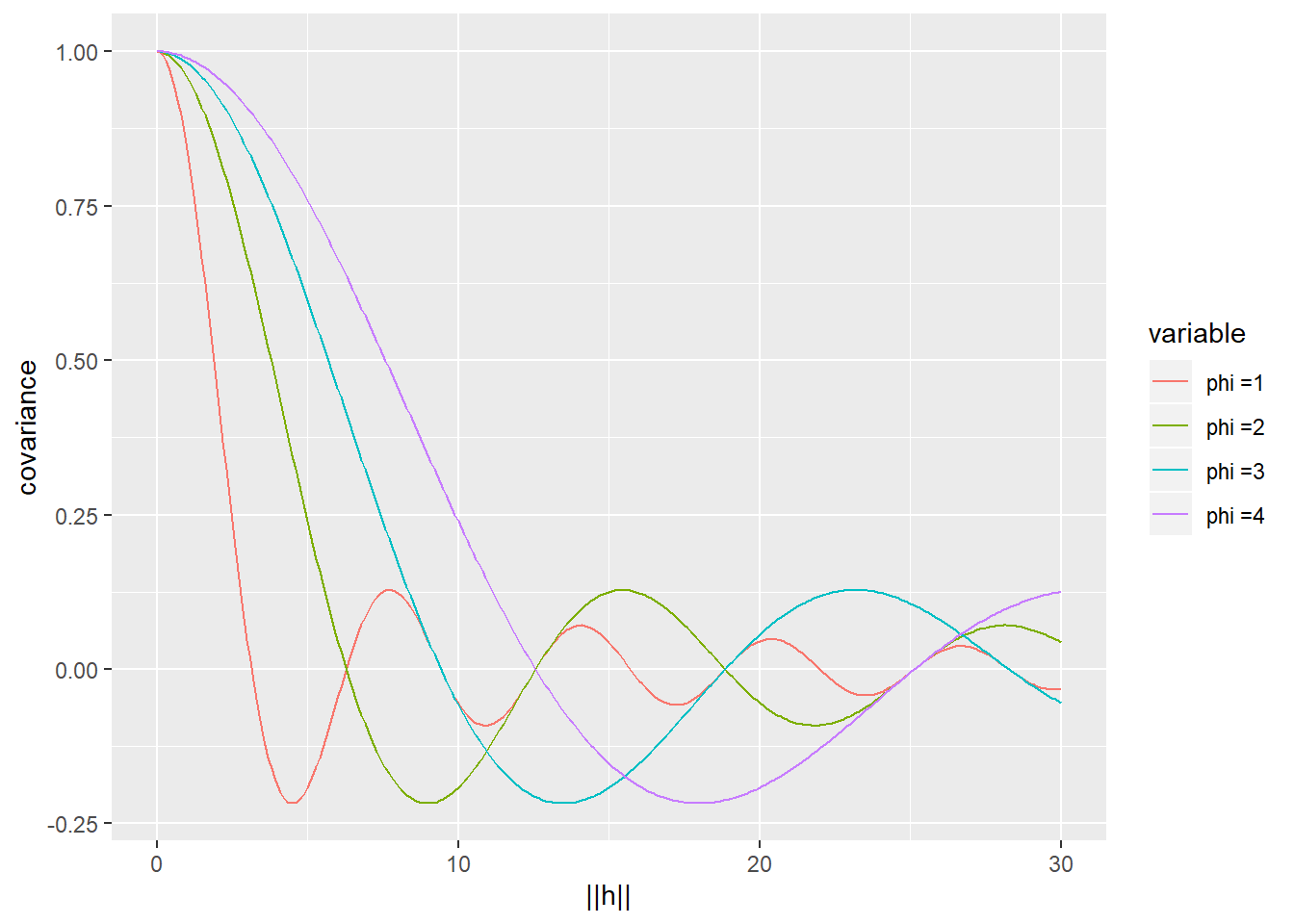
The Matérn covariance function \(C(h|\sigma^2, \phi,\nu)\), where \(\sigma^2 > 0, \phi>0,\nu>0\) are marginal variance, range and smoothness parameters, is widely used to model covariance structures in spatial statistics. It is defined as \[C({\mathbf{h}}|\sigma^2, \phi,\nu):=\frac{2^{1-\nu}\sigma^2}{\Gamma(\nu)}(||{\mathbf{h}}||/\phi)^\nu K_\nu(||{\mathbf{h}}||/\phi),\] where \(K_\nu\) is a modified Bessel function of the second kind (see, e.g., N. Cressie (1993), Schabenberger and Gotway (2017)).

1. The Matérn covariance function is isotropic. The correlation decreases when the distance \(||h||\) increases.

2. When \(\nu\) increases, the smoothness of the random field increases. As \(\nu\to \infty\), the limiting covariance function is known as gaussian model \[C({\mathbf{h}}) = \sigma^2 \exp(-||h||^2/\phi),\] which leads to an infinitely differentiable random field. Usually physical and biological processes are not so smooth.

3. If \(\nu = 0.5\), the resulting model is well known as exponential covariance function, \[C({\mathbf{h}}) = \sigma^2 \exp(-||{\mathbf{h}}||/\phi).\] In geostatistical application, the range of a spatial model means the distance at which the correlations have decreased to \(\approx 0.05\) or less. Here, solving \(\exp(-||h||/\phi) = 0.05\), we get \(||h|| = -\phi\log(0.05)\). Thus, \(\phi\) is called range parameter. However, for any fixed \(\nu\), the range of a Matérn model is a function of \(\phi\) and \(\nu\).

The plot below shows Matérn covariance functions with varying \(\nu\)s.

3.1.2 Some other common covariance functions

1. Spherical: For spatial data in \(1D\), \(2D\) or \(3D\), spherical covariance function is given by \[C({\mathbf{h}}) =\left\{\begin{array}{ll} 1-\frac{3}{2}\frac{||{\mathbf{h}}||}{\phi} + \frac{1}{2}\left(\frac{||{\mathbf{h}}||}{\phi}\right)^3, & ||{\mathbf{h}}|| \leq \phi\\ 0,&\text{otherwise}. \end{array} \right.\]

2. Powered exponential: As a generalization of exponential model, powered exponential covariance is given by

\[C({\mathbf{h}}) =\sigma^2 \exp(-||{\mathbf{h}}||^\nu/\phi^\nu),\] where \(\nu \in (0,2]\) and \(\phi > 0\).

3. “Generalized Cauchy”: The Cauchy covariance is given by

\[C({\mathbf{h}}) = \sigma^2 (1+(||{\mathbf{h}}||^\nu/\phi^\nu))^{-\beta/\nu},\] where \(\nu \in (0,2]\), \(\phi > 0\) and \(\beta > 0\).

4. Wave (cardinal-sine or hole-effect): The wave covariance function is given by \[C({\mathbf{h}}) = \sigma^2 \phi/||{\mathbf{h}}||\sin(||{\mathbf{h}}||/\phi),\] where \(\phi > 0\).

3.1.3 Geometric anisotropy

If the covariance function of a weakly stationary random field is anisotropic, the spatial structure is direction dependent. A commonly used class of anisotropic covariance functions is the geometric anisotropic covariance functions, which can be corrected by a linear transformation of the coordinate system. Let \(Y_1({\mathbf{s}})\) be an isotropic random field in \({\mathbb{R}}^d\) with mean \(\mu\) and covariance \(C_1({\mathbf{h}})=f(||{\mathbf{h}}||)\) and let \(B\) be \(d\times d\) nonsingular matrix. Define \[Y({\mathbf{s}}) = Y_1(B{\mathbf{s}}).\] Then we know \({\mathbb{E}}(Y({\mathbf{s}})) = \mu\) and \[{\text{Cov}}(Y({\mathbf{s}}),Y({\mathbf{s}}+{\mathbf{h}})) = {\text{Cov}}(Y_1(B{\mathbf{s}}),Y_1(B{\mathbf{s}}+{\mathbf{h}})) = C_1(Bh)=f(||Bh||)=f({\mathbf{h}}^\top W {\mathbf{h}})\equiv C({\mathbf{h}}),\] where \(W = B^\top B\). Here, \(C({\mathbf{h}})\) is a geometrically anisotropic covariance function.

To correct for geometric anisotropy, the transformation of the coordinate can be reversed. Let \({\mathbf{s}}=(sx,sy)^\top\) be the coordinate in \({\mathbb{R}}^2\) such that \(Y({\mathbf{s}})\) is geometrically anisotropic. Then the linear transformation \({\mathbf{s}}^* = B^{-1}{\mathbf{s}}\) transform \({\mathbf{s}}\) back to isotropic space. \(B^{-1}\) can be represented by \[B^{-1} =\begin{pmatrix} 1&0\\ 0&\lambda \end{pmatrix} \begin{pmatrix} \cos(\theta) & -\sin(\theta)\\ \sin(\theta) & \cos(\theta) \end{pmatrix}, \] where \(\lambda\) is the anisotropy ratio and \(\theta\) is the rotation angle. Recall the anisotropic anisotropic Matérn covariance function plot in chapter 2.

3.1.4 Semivariogram

There is a third type of stationarity called intrinsic stationary. A random field \(Y({\mathbf{s}})\) is intrinsic stationary if \({\mathbb{E}}(Y({\mathbf{s}})) = \mu\) and \[\frac{1}{2}{\text{Var}}(Y({\mathbf{s}}+h)-Y({\mathbf{s}})) = \gamma({\mathbf{h}}).\] The function \(\gamma({\mathbf{h}})\) is called semivariogram of the random field and \(2\gamma({\mathbf{h}})\) is called variogram.

The semivariogram is conditional negative definite, that is, for all \(n\), all \({\mathbf{s}}_1,...,{\mathbf{s}}_n\), and all \(a_1,...,a_n\) such that \(\sum_{i=1}^n a_i=0\), we have \[\sum_{i,j=1}^n a_ia_j \gamma({\mathbf{s}}_i-{\mathbf{s}}_j) \leq 0.\]

Note that if \(Y({\mathbf{s}})\) is weakly stationary, then

\[{\text{Var}}(Y({\mathbf{s}}) - Y({\mathbf{s}}+{\mathbf{h}})) = {\text{Var}}(Y({\mathbf{s}})) + {\text{Var}}(Y({\mathbf{s}}+{\mathbf{h}})) - 2{\text{Cov}}(Y({\mathbf{s}}), Y({\mathbf{s}}+{\mathbf{h}})) = 2(C(\mathbf{0})-C({\mathbf{h}})).\] Hence, any weakly stationary random field is also intrinsic stationary. Further, we can see that if \(C({\mathbf{h}})\) decreases with increasing \(||{\mathbf{h}}||\), \(\gamma({\mathbf{h}})\) will approach \(C(0) = \sigma^2\) either asymptotically or exactly at a particular lag \(h^*\). \(\sigma^2\) is called the sill of the semivariogram and the lag \({\mathbf{h}}^*\) at which the sill is reached is called its range. If the sill is reached asymptotically, the practical range is defined as the lag \({\mathbf{h}}^*\) at which \(\gamma({\mathbf{h}}) = 0.95\sigma^2\).

However, intrinsic stationarity does not imply weakly stationarity. As an example, the power model is intrinsic stationary but not weakly stationary. It is given in terms of the semivariogram \[\gamma({\mathbf{h}}) = \theta ||{\mathbf{h}}||^\lambda,\] where \(\theta > 0\) and \(\lambda \in [0,2)\). Since \(\gamma({\mathbf{h}}) \to \infty\) as \(||{\mathbf{h}}|| \to \infty\), the power model is not weakly stationary.

3.2 Spatial models without predictors

In this section, we’ll consider models for the geostatistical data \(y({\mathbf{s}}_1),..., y({\mathbf{s}}_n)\) without any predictors. In other words, to learn the underlying true random field \(Y({\mathbf{s}}), {\mathbf{s}}\in \mathcal{D}\), the only sample we have are those \(n\) data points and their coordinates.

Let’s start with an example from Schabenberger and Gotway (2017).

Example 3.1 (C/N ratios) In a study, the total carbon (TC) and total soil nitrogen (TN) percentages were measured at 195 locations on an agriculture fields. Further, the C/N ratios were obtained by calculating the ratio of TC to TN. One of the research goals is to bulid up a model to predict the C/N ratios beyond those 195 locations. The data is included in “CNRatio.csv”

To explore the spatial pattern, we can use an interpolated 2D plot to display the data. The plot below suggests some degree of spatial dependence.

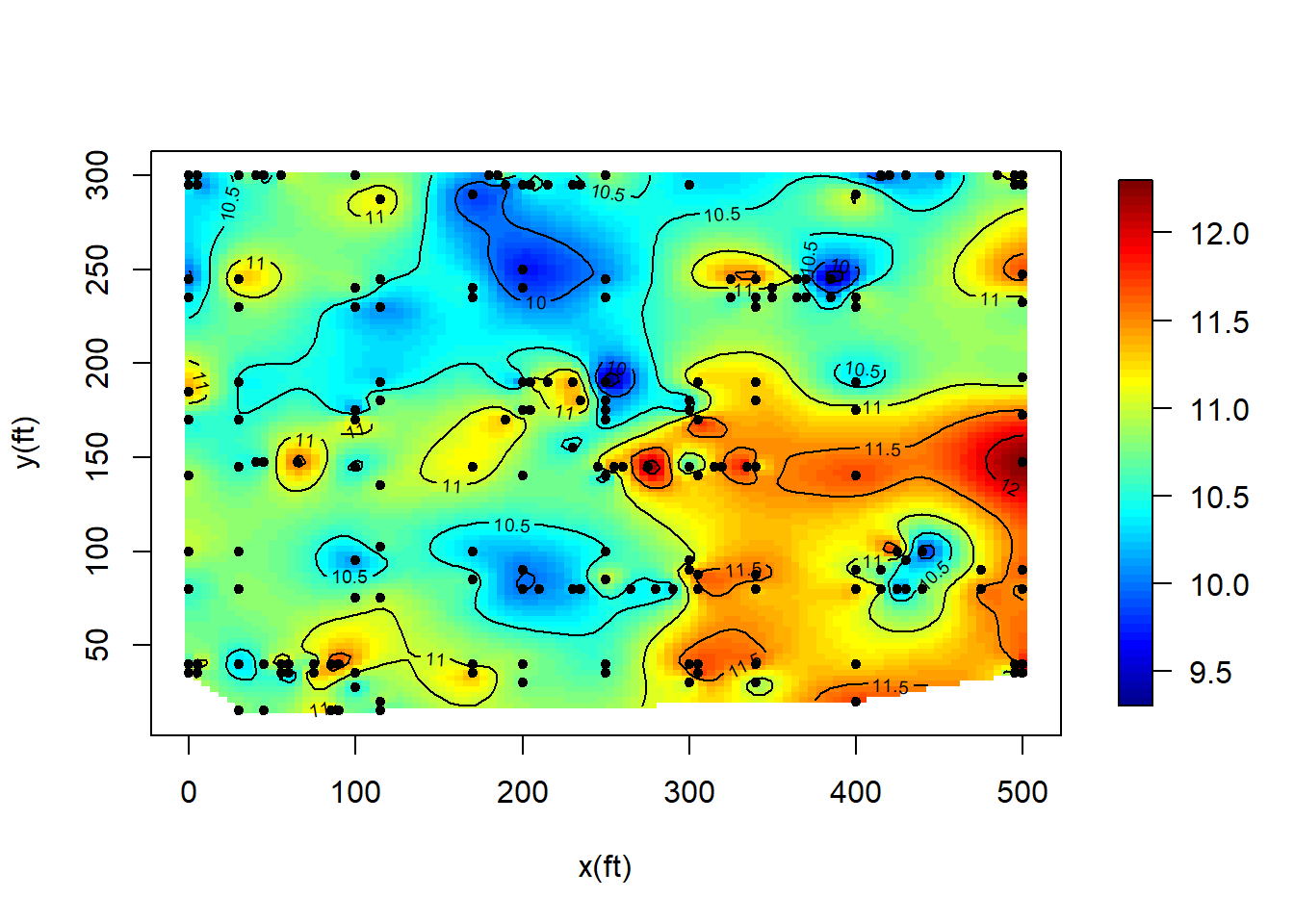
Let \(Y({\mathbf{s}})\) be the C/N ratio at location \({\mathbf{s}}\). Since there are no other predictors, a reasonable model we can try is \[Y({\mathbf{s}}) = \mu + w({\mathbf{s}}) + e({\mathbf{s}}),\] where \(\mu\) is unknown constant mean, \(w({\mathbf{s}})\) is a weakly stationary random field with mean zero and covariance function \(C_w({\mathbf{h}})\) and \(e({\mathbf{s}})\) is a white noise with variance \(\sigma_e^2\).

Hence, the covariance function of \(Y({\mathbf{s}})\) is \[C_Y({\mathbf{h}}) = \left\{ \begin{array}{ll} C_w({\mathbf{h}}) & \text{if}\ {\mathbf{h}}\neq \mathbf{0}\\ C_w(\mathbf{0}) + \sigma_e^2 & \text{if}\ {\mathbf{h}}= \mathbf{0} \end{array} \right.,\] and the semivariogram of \(Y({\mathbf{s}})\) is \(\gamma_Y({\mathbf{h}}) = C_Y(\mathbf{0}) - C_Y({\mathbf{h}})\).

Usually, we’ll use a parametric positive definite function to model \(C_w({\mathbf{h}})\). Suppose that we use an exponential covariance function, that is \(C_w({\mathbf{h}}) = \sigma_w^2 \exp(-||{\mathbf{h}}||/\phi).\)

Let \({\mathbf{Y}}=(y(s_1), ..., y({\mathbf{s}}_n))^\top\), \(\text{Var}({\mathbf{Y}}) = \Sigma\), and \({\boldsymbol{\epsilon}}= (w({\mathbf{s}}_1)+e({\mathbf{s}}_1), ..., w({\mathbf{s}}_n)+e({\mathbf{s}}_n))^\top\). Then the data model is \[{\mathbf{Y}}= \mathbf{1}\mu + {\boldsymbol{\epsilon}}.\] For model estimations, we are expected to find estimators of \(\mu, \sigma_w^2, \phi\), and \(\sigma_e^2\). There are three main methods for estimations, that are variogram methods (classical geostatistical methods), maximum likelihood estimations (MLE) and restricted maximum likelihood (REML) estimations.

3.2.1 Spatial estimations

1. Variogram methods

In Chapter 1&2, we’ve derived that the BLUE of \(\mu\) is the generalized linear estimator, \[\hat \mu_{gls} = (\mathbf{1}^\top \Sigma^{-1}\mathbf{1})^{-1}(\mathbf{1}^\top \Sigma^{-1}{\mathbf{Y}}).\] Here, \(\Sigma\) is determined by the covariance function \(C_Y({\mathbf{h}})\) or the variogram \(\gamma_Y({\mathbf{h}})\), which is determined by \(\sigma_w^2, \phi\), and \(\sigma_e^2\). So if we can first estimate \(\sigma_w^2, \phi\), and \(\sigma_e^2\), then \(\hat \mu_{egls}\) can be obtained by plugging \(\hat \Sigma\) to \(\Sigma\) in \(\hat \mu_{gls}\).

To this end, we first introduce empirical estimations of the variogram \(\gamma_Y({\mathbf{s}})\).

Matheron estimator: \[\hat \gamma_Y({\mathbf{h}}) = \frac{1}{2|N({\mathbf{h}})|} \sum_{N({\mathbf{h}})}\{y({\mathbf{s}}_i)-y({\mathbf{s}}_j)\}^2,\] where \(N({\mathbf{h}}) = \{({\mathbf{s}}_i,{\mathbf{s}}_j)\, |\, {\mathbf{s}}_i-{\mathbf{s}}_j = {\mathbf{h}}\}\) and \(|N({\mathbf{h}})|\) denotes the number of distinct pairs in \(N({\mathbf{h}})\). Typically, at least \(30\) pairs of locations should be available at each lag. However, when the sample size \(n\) is small or the data are irregularly shaped, \(|N({\mathbf{h}})|\) for given \({\mathbf{h}}\) might be too small to provide a stable estimate at lag \({\mathbf{h}}\). For isotropic semivariogram, a method to fix this is averaging the squared differences on the set \[N^*({\mathbf{h}},\epsilon) = \{({\mathbf{s}}_i,{\mathbf{s}}_j)\ |\ ||{\mathbf{s}}_i-{\mathbf{s}}_j|| \in (||{\mathbf{h}}||-\epsilon, ||{\mathbf{h}}||+\epsilon)\},\] where \(\epsilon\) is the user tolerance. For general semivariograms, a partition of the lag space \(H = \{{\mathbf{s}}-{\mathbf{s}}':\, {\mathbf{s}},{\mathbf{s}}' \in \mathcal{D}\) into lag classes (or “bins”) is necessary.

Remark: i). The advantage of estimating \(\gamma_Y({\mathbf{h}})\) over estimating \(C({\mathbf{h}})\) stems from the fact that the unknown mean \(\mu\) is filtered in semivariogram when the mean is constant.

ii). It it not recommended to compute \(\hat \gamma_Y({\mathbf{h}})\) up to the largest possible lag class. A common recommendation is to compute it up to about one half of the maximum separation distance in the data.

iii). Matheron estimator is sensitive to outliers because the squared differences magnify the deviation between an outlier and other values. A robust estimator, Cressie-Hawkins estimator, was proposed to address this issue. It is given by \[\tilde \gamma_Y({\mathbf{h}}) = \frac{\left(\frac{1}{|N({\mathbf{h}})|} \sum_{N({\mathbf{h}})}\{y({\mathbf{s}}_i)-y({\mathbf{s}}_j)\}^{0.5}\right)^4}{0.914+0.988/|N({\mathbf{h}})|}.\]

Now we estimate \(\gamma_Y({\mathbf{h}})\) in Example 3.1 in R.

rm(list=ls())
library(MBA)
library(fields)
dat <- read.csv("./data/CNRatio.csv", header = TRUE) 
s <- dat[,1:2]#coordinates
CN <- dat[,5]#CNRatio
#estimate gamma(h)
library(spBayes)
library(geoR)
max.dist <-  0.5 * max(iDist(s))
bins <- 100
#Matheron estimator
vario.CN.M <- variog(coords = s, data = CN, estimator.type = "classical",
                     uvec = (seq(0, max.dist, l = bins )))

## variog: computing omnidirectional variogram

#Cressie-Hawkins estimator
vario.CN.CH <- variog(coords = s, data = CN, estimator.type = "modulus",
                      uvec = (seq(0, max.dist, l = bins )))

## variog: computing omnidirectional variogram

plot(vario.CN.M, main = "CNRatios")
points(vario.CN.CH$u, vario.CN.CH$v, col = "red")
legend("bottomright", legend=c("Matheron", "Cressie-Hawkins"), 
       pch = c(1,1), col = c("black", "red"), cex = 0.6)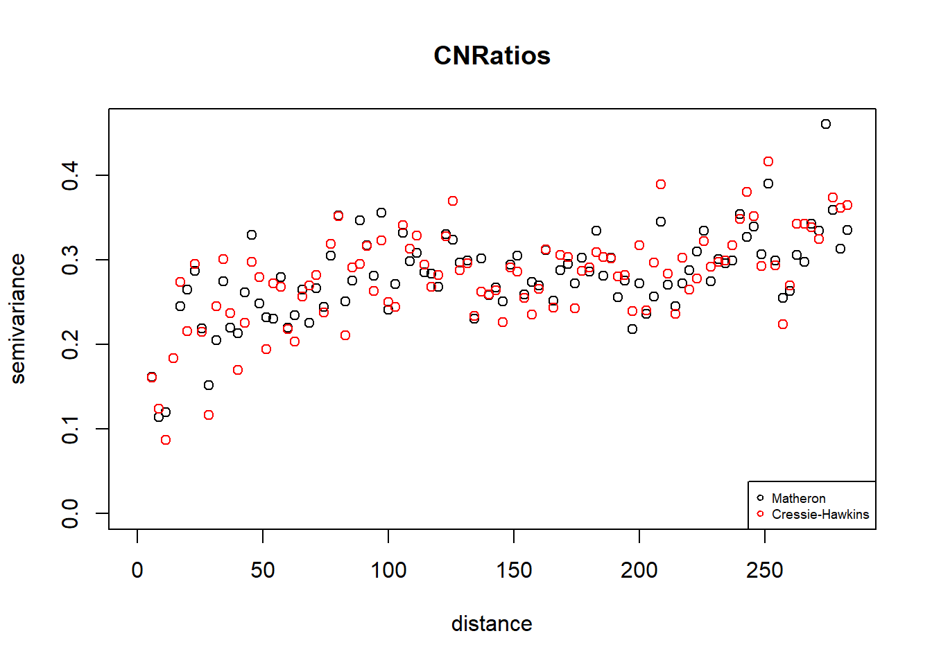

We’ve got the estimator of semivariogram \(\hat \gamma_Y({\mathbf{h}})\) or \(\tilde \gamma_Y({\mathbf{h}})\). Suppose that we chose \(k\) bins and obtained \(\hat \gamma_Y({\mathbf{h}})\) or \(\tilde \gamma_Y({\mathbf{h}})\) at \({\mathbf{h}}_1,...,{\mathbf{h}}_k\). Then, the parametric semivariogram \(\gamma_Y({\mathbf{h}})\) can be fit to the pseudo-data \[\hat \gamma_Y({\mathbf{h}}) = (\hat \gamma_Y({\mathbf{h}}_1),..., \hat \gamma_Y({\mathbf{h}}_k))^\top,\] or \[\tilde \gamma_Y({\mathbf{h}}) = (\tilde \gamma_Y({\mathbf{h}}_1),..., \tilde \gamma_Y({\mathbf{h}}_k))^\top.\] In the following we focus on the Matheron estimator \(\hat \gamma_Y({\mathbf{h}})\). To emphasize \(\gamma_Y({\mathbf{h}})\) is a parametric semivariogram, we denote its values at \({\mathbf{h}}_1,...,{\mathbf{h}}_k\) by \[\gamma_Y({\mathbf{h}};{\boldsymbol{\theta}}) = (\gamma_Y({\mathbf{h}}_1;{\boldsymbol{\theta}}),...,\gamma_Y({\mathbf{h}}_k;{\boldsymbol{\theta}}))^\top.\] In Example 3.1, we use exponential covariance function and hence \({\boldsymbol{\theta}}= (\phi, \sigma_w^2, \sigma_e^2)\). Since it is easy to check \({\mathbb{E}}(\hat \gamma_Y({\mathbf{h}}) = \gamma_Y({\mathbf{h}};{\boldsymbol{\theta}})\), to estimate \({\boldsymbol{\theta}}\), we consider the following linear model \[\hat \gamma_Y({\mathbf{h}}) = \gamma_Y({\mathbf{h}};{\boldsymbol{\theta}}) + {\boldsymbol{\epsilon}}({\mathbf{h}}),\] where \({\boldsymbol{\epsilon}}({\mathbf{h}})\) are just the difference between \(\hat \gamma_Y({\mathbf{h}})\) and \(\gamma_Y({\mathbf{h}};{\boldsymbol{\theta}})\). Suppose that \({\text{Var}}(\hat \gamma_Y({\mathbf{h}})) = V({\boldsymbol{\theta}})\), which typically depends on \({\boldsymbol{\theta}}\). Then \(\hat {\boldsymbol{\theta}}\) can be obtained by solving a standard nonlinear generalized least square problems, \[\min_{{\boldsymbol{\theta}}} (\hat \gamma_Y({\mathbf{h}}) - \gamma_Y({\mathbf{h}};{\boldsymbol{\theta}}))^\top V({\boldsymbol{\theta}})^{-1}(\hat \gamma_Y({\mathbf{h}}) - \gamma_Y({\mathbf{h}};{\boldsymbol{\theta}})).\] \(\hat {\boldsymbol{\theta}}\) obtained from the above procedure is efficient. However, it is challenging to get the form of \(V({\boldsymbol{\theta}})\). In practice, an approximations on the diagonals of \(V({\boldsymbol{\theta}})\) were derived under Gaussian assumptions, that is \[{\text{Var}}(\hat \gamma_Y({\mathbf{h}}_i)) \approx 2 \frac{\gamma_Y^2({\mathbf{h}}_i;{\boldsymbol{\theta}})}{|N(h_i)|}, i= 1,2,...,k.\] and then \(V({\boldsymbol{\theta}})\) is replaced by its diagonal matrix, say \(W({\boldsymbol{\theta}})\). Finally, \({\boldsymbol{\theta}}\) are estimated via a weighted least squares (WLS) approach, that is \[\min_{{\boldsymbol{\theta}}} (\hat \gamma_Y({\mathbf{h}}) - \gamma_Y({\mathbf{h}};{\boldsymbol{\theta}}))^\top W({\boldsymbol{\theta}})^{-1}(\hat \gamma_Y({\mathbf{h}}) - \gamma_Y({\mathbf{h}};{\boldsymbol{\theta}}))= \sum_{i=1}^k \frac{|N(h_i)|}{2\gamma_Y^2({\mathbf{h}}_i;{\boldsymbol{\theta}})}(\hat \gamma_Y({\mathbf{h}}_i)-\gamma_Y({\mathbf{h}}_i;\theta))^2.\] In Example 3.1, \[\gamma_Y({\mathbf{h}};{\boldsymbol{\theta}}) = \left\{ \begin{array}{ll} \sigma_e^2+\sigma_w^2(1-e^{-||{\mathbf{h}}||/\phi}),& \text{if}\ {\mathbf{h}}\neq 0\\ 0,&\text{if}\ {\mathbf{h}}= 0. \end{array}\right.\]

Also, in practice, people may just use \(|N(h_i)|\) rather than \(\frac{|N(h_i)|}{2\gamma_Y^2({\mathbf{h}}_i;{\boldsymbol{\theta}})}\) as weights, or even set all weights equal to one. But the WLS approach is still preferred since it assigns relatively less weight to \(\hat \gamma_Y({\mathbf{h}}_i)\) with large lag \({\mathbf{h}}_i\).

Now we’ll estimate \({\boldsymbol{\theta}}\) using R.

#OLS with "nls"
variofit(vario.CN.M, ini.cov.pars = c(var(CN),
-max.dist/log(0.05)),cov.model = "exponential",minimisation.function
= "nls", weights = "equal", messages = FALSE)

## variofit: model parameters estimated by OLS (ordinary least squares):
## covariance model is: exponential
## parameter estimates:
##   tausq sigmasq     phi 
##  0.1319  0.1675 37.7832 
## Practical Range with cor=0.05 for asymptotic range: 113.1883
## 
## variofit: minimised sum of squares = 0.1574

#OLS with "optim"
variofit(vario.CN.M, ini.cov.pars = c(var(CN),
-max.dist/log(0.05)),cov.model = "exponential",minimisation.function
= "optim", weights = "equal",
control = list(factr=1e-8, maxit = 500), messages = FALSE)#use "L-BFGS-B"

## variofit: model parameters estimated by OLS (ordinary least squares):
## covariance model is: exponential
## parameter estimates:
##   tausq sigmasq     phi 
##  0.1319  0.1675 37.7830 
## Practical Range with cor=0.05 for asymptotic range: 113.1876
## 
## variofit: minimised sum of squares = 0.1574

#WLS with weights N(h)
variofit(vario.CN.M, ini.cov.pars = c(var(CN), -max.dist/log(0.05)),cov.model = "exponential",
 minimisation.function = "optim", weights = "npairs", 
 control = list(factr=1e-10, maxit = 500), messages = FALSE)

## variofit: model parameters estimated by WLS (weighted least squares):
## covariance model is: exponential
## parameter estimates:
##   tausq sigmasq     phi 
##  0.1655  0.1355 54.1686 
## Practical Range with cor=0.05 for asymptotic range: 162.2745
## 
## variofit: minimised weighted sum of squares = 19.981

#WLS with weights N(h)/gamma^2(h)
variofit(vario.CN.M, ini.cov.pars = c(var(CN), -max.dist/log(0.05)),cov.model = "exponential",
minimisation.function = "optim", weights = "cressie", 
control = list(factr=1e-10, maxit = 500), messages = FALSE)

## variofit: model parameters estimated by WLS (weighted least squares):
## covariance model is: exponential
## parameter estimates:
##   tausq sigmasq     phi 
##  0.2035  0.1144 94.4488 
## Practical Range with cor=0.05 for asymptotic range: 282.9434
## 
## variofit: minimised weighted sum of squares = 247.3375

So far, we’ve introduced the variogram methods to estimate the spatial model parameters. The methods are popular in practice because of its simplicity. It is widely used in exploratory data analysis. However, although the procedure yields consistent and asymptotically normal estimators \(\hat {\boldsymbol{\theta}}\) under certain regularity conditions (see, Lahiri, Lee, and Cressie (2002)), it is suboptimal and does not rest on as firm theoretical footing as the likelihood-based approaches (A. Gelfand et al. (2010)).

2. Maximum likelihood estimations (MLE)

Assume that \(Y({\mathbf{s}})\) is a Gaussian random field. We can apply the MLE method in Section 2.4 to estimate \({\boldsymbol{\theta}}= (\sigma_w^2, \phi, \sigma_e^2)\) and \(\mu\), which can be obtained by maximizing the following log likelihood function \[\log \ell(\mu,{\boldsymbol{\theta}}; {\mathbf{Y}}) = -\frac{n}{2}\log(2\pi)-\frac{1}{2}\log|\Sigma({\boldsymbol{\theta}})| - \frac{1}{2}({\mathbf{Y}}-\mathbf{1}\mu)^\top \Sigma^{-1}({\boldsymbol{\theta}})({\mathbf{Y}}-\mathbf{1}\mu).\]

Here are some Remarks from A. Gelfand et al. (2010).

i). There are no guarantee of existence or uniqueness, nor is there even a guarantee that all local maxima of the likelihood function are global maxima. For example, the likelihood with spherical covariance often has multiple modes.

ii). Multiple modes are extremely rare in practice for Matérn covariance functions, such as the exponential function.

iii). A reasonably practical strategy for determining whether a local maximum obtained by an iterative algorithm is likely to be the unique global maximum is to repeat the algorithm from several widely dispersed starting values.

Now we apply MLE method to Example 3.1 in R.

#MLE
fit.mle <- likfit(coords = s, data = CN, trend = "cte", ini.cov.pars =
c(var(CN), -max.dist/log(0.05)), cov.model = "exponential",
lik.method = "ML", control = list(factr=1e-10, maxit = 500))

## kappa not used for the exponential correlation function
## ---------------------------------------------------------------
## likfit: likelihood maximisation using the function optim.
## likfit: Use control() to pass additional
##          arguments for the maximisation function.
##         For further details see documentation for optim.
## likfit: It is highly advisable to run this function several
##         times with different initial values for the parameters.
## likfit: WARNING: This step can be time demanding!
## ---------------------------------------------------------------
## likfit: end of numerical maximisation.

print(fit.mle)

## likfit: estimated model parameters:
##      beta     tausq   sigmasq       phi 
## "10.8507" " 0.1132" " 0.2023" "47.0144" 
## Practical Range with cor=0.05 for asymptotic range: 140.8424
## 
## likfit: maximised log-likelihood = -131.2

#try different initial values
ini <- matrix(c(seq(0.05,1,l=10), seq(10, 200, l = 10)), ncol = 2)
fit <- sapply(1:10, function(m) {fit <- likfit(coords = s, data = CN,
      trend = "cte", ini.cov.pars = ini[m,], cov.model = "exponential",
      lik.method = "ML", control = list(factr=1e-10, maxit = 500),
      messages = FALSE); return(c(fit$nugget, fit$cov.pars))})
print(t(fit))

##            [,1]      [,2]     [,3]
##  [1,] 0.1131637 0.2023052 47.01435
##  [2,] 0.1131637 0.2023052 47.01435
##  [3,] 0.1131637 0.2023052 47.01435
##  [4,] 0.1131637 0.2023052 47.01435
##  [5,] 0.1131637 0.2023052 47.01435
##  [6,] 0.1131637 0.2023053 47.01437
##  [7,] 0.1131636 0.2023053 47.01434
##  [8,] 0.1131637 0.2023052 47.01437
##  [9,] 0.1131636 0.2023053 47.01433
## [10,] 0.1131637 0.2023052 47.01435

3. Restricted maximum likelihood estimations (REML)

MLEs are asymptotically Gaussian and efficient. However, in finite samples, the MLEs of variance and covariance parameters, such as \(\sigma_w^2\), \(\sigma_e^2\) and \(\phi\) in Example 3.1, are often negatively biased.

Consider the linear model \[\begin{align} \mathbf{Y} = \mathbf{X} \boldsymbol{\beta} + \boldsymbol{\epsilon}, \end{align}\]

where \({\mathbb{E}}({\boldsymbol{\epsilon}}) = \mathbf{0}\) and \(\text{Var}({\boldsymbol{\epsilon}}) = \Sigma({\boldsymbol{\theta}})\).

The bias is due to the fact of “loss in degrees of freedom” from estimating \({\boldsymbol{\beta}}\). Restricted (or residual) maximum likelihood (REML) estimations reduce the bias in MLEs.

Suppose that the rank of \({\mathbf{X}}\) is \(q\). The idea of REML estimation is to estimate variance and covariance parameters by maximizing the likelihood of \(K{\mathbf{Y}}\), where \(K\) is \((n-q)\times n\) matrix such that for any \({\boldsymbol{\beta}}\in {\mathbb{R}}^p\), \[{\mathbb{E}}(K{\mathbf{Y}}) = K{\mathbf{X}}{\boldsymbol{\beta}}= \mathbf{0}.\] \(K\) is called a matrix of error contrasts. It is equivalent to require \(K{\mathbf{X}}=\mathbf{0}\). Multiplying \(K\) on both sides of the linear model above, we have \[K\mathbf{Y} = K\boldsymbol{\epsilon}\]

Then, the log likelihood function of \(K{\mathbf{Y}}\) is \[\log \ell({\boldsymbol{\theta}}; {\mathbf{Y}}) = -\frac{n-q}{2}\log(2\pi)-\frac{1}{2}\log|K\Sigma({\boldsymbol{\theta}})K^\top| - \frac{1}{2}{\mathbf{Y}}^\top K^\top \Sigma^{-1}({\boldsymbol{\theta}})K{\mathbf{Y}}.\]

In Example 3.1, since the mean is constant, it is easy to obtain the \((n-1)\times n\) matrix \[K = \begin{pmatrix} 1-1/n & -1/n &\cdots &-1/n& -1/n\\ -1/n & 1-1/n & \cdots & -1/n&-1/n\\ \vdots & \vdots & \ddots &\vdots& \vdots\\ -1/n & -1/n &\cdots & 1-1/n&-1/n\\ \end{pmatrix}.\]

Let \(\hat{\boldsymbol{\theta}}_{reml}\) be the REML estimators. The mean \(\mu\) can be obtained by

\[(\mathbf{1}^\top \Sigma^{-1}(\hat{\boldsymbol{\theta}}_{reml})\mathbf{1})^{-1}\mathbf{1}^\top \Sigma^{-1}(\hat{\boldsymbol{\theta}}_{reml}){\mathbf{Y}}.\] Now we apply REML estimations to Example 3.1.

#REML
fit.reml <- likfit(coords = s, data = CN, trend = "cte", ini.cov.pars =
         c(var(CN), -max.dist/log(0.05)), cov.model = "exponential",
       lik.method = "REML", control = list(factr=1e-10, maxit = 500))

## kappa not used for the exponential correlation function
## ---------------------------------------------------------------
## likfit: likelihood maximisation using the function optim.
## likfit: Use control() to pass additional
##          arguments for the maximisation function.
##         For further details see documentation for optim.
## likfit: It is highly advisable to run this function several
##         times with different initial values for the parameters.
## likfit: WARNING: This step can be time demanding!
## ---------------------------------------------------------------
## likfit: end of numerical maximisation.

print(fit.reml)

## likfit: estimated model parameters:
##      beta     tausq   sigmasq       phi 
## "10.8594" " 0.1180" " 0.2159" "57.0518" 
## Practical Range with cor=0.05 for asymptotic range: 170.912
## 
## likfit: maximised log-likelihood = -129.8

#try different initial values
ini <- matrix(c(seq(0.05,1,l=10), seq(10, 200, l = 10)), ncol = 2)
fit <- sapply(1:10, function(m) {fit <- likfit(coords = s, data = CN,
trend = "cte", ini.cov.pars = ini[m,], cov.model = "exponential", lik.method = "REML", 
control = list(factr=1e-10, maxit = 500), messages = FALSE);
return(c(fit$nugget, fit$cov.pars))})
print(t(fit))

##            [,1]      [,2]     [,3]
##  [1,] 0.1180445 0.2159133 57.05183
##  [2,] 0.1180445 0.2159132 57.05182
##  [3,] 0.1180445 0.2159133 57.05183
##  [4,] 0.1180445 0.2159132 57.05182
##  [5,] 0.1180445 0.2159132 57.05182
##  [6,] 0.1180445 0.2159132 57.05181
##  [7,] 0.1180444 0.2159133 57.05176
##  [8,] 0.1180445 0.2159132 57.05182
##  [9,] 0.1180445 0.2159132 57.05182
## [10,] 0.1180445 0.2159132 57.05182

Here are some Remarks from A. Gelfand et al. (2010).

i). The negative bias of MLE on variance and covariance parameters lead to overly optimistic inferences on mean parameters and predictions. Especially, when the number of predictors \(p\) is large relative to \(n\), MLEs may be considerably underestimated.

ii). REML does reduce bias, but it may increase estimation variance.

iii). In applications, whether prefer ML to REML estimations depends on which problem one considers to be more serious.

3.2.2 Spatial prediction (Kriging)

One of the pervasive problems in spatial statistics is to predict the values of the random field \(Y\) at desired locations. Geostatistical prediction methods to this purpose are called kriging, after the South African mining engineer D. G. Krige, who was first to develop and apply them. If the mean function is assumed to be constant, that is \[Y({\mathbf{s}}) = \mu + w({\mathbf{s}}) + e({\mathbf{s}}),\] then the prediction method is called ordinary kriging, which actually is the best linear unbiased prediction.

Let \[{\mathbf{c}}({\boldsymbol{\theta}})={\text{Cov}}({\mathbf{Y}}, Y({\mathbf{s}}_0)) = (C_Y({\mathbf{s}}_1-{\mathbf{s}}_0;{\boldsymbol{\theta}}),...,C_Y({\mathbf{s}}_n-{\mathbf{s}}_0;{\boldsymbol{\theta}}))^\top,\] and let \[\Sigma({\boldsymbol{\theta}}) = {\text{Var}}({\mathbf{Y}}) = (C_Y({\mathbf{s}}_i-{\mathbf{s}}_j;{\boldsymbol{\theta}}))_{i,j=1}^n.\] Note that both \({\mathbf{c}}({\boldsymbol{\theta}})\) and \(\Sigma({\boldsymbol{\theta}})\) depends on the unknown \({\boldsymbol{\theta}}\), the parameters of the covariance function. In Chapter \(1\) Example 1.5, we derived the BLUP of this type of model with a specific covariance structure. In general, the BLUP of \(Y\) at location \({\mathbf{s}}_0\) can be written as, \[\hat Y({\mathbf{s}}_0) = \hat \mu_{gls}({\boldsymbol{\theta}}) + {\mathbf{c}}({\boldsymbol{\theta}})^\top\Sigma({\boldsymbol{\theta}})^{-1}({\mathbf{Y}}-\mathbf{1}\hat \mu_{gls}({\boldsymbol{\theta}})),\] where \[\hat \mu_{gls}({\boldsymbol{\theta}}) = (\mathbf{1}^\top \Sigma({\boldsymbol{\theta}})^{-1}\mathbf{1})^{-1}(\mathbf{1}^\top \Sigma({\boldsymbol{\theta}})^{-1}{\mathbf{Y}}).\] The variance of \(\hat Y({\mathbf{s}}_0)\) is \[{\text{Var}}(\hat Y({\mathbf{s}}_0)) = C_Y(\mathbf{0}) - {\mathbf{c}}({\boldsymbol{\theta}})^\top \Sigma({\boldsymbol{\theta}})^{-1}{\mathbf{c}}({\boldsymbol{\theta}}) + (1-\mathbf{1}^\top \Sigma({\boldsymbol{\theta}})^{-1}{\mathbf{c}}({\boldsymbol{\theta}}))^2(\mathbf{1}^\top \Sigma({\boldsymbol{\theta}})^{-1}\mathbf{1})^{-1}.\] To get the prediction, we have to substitute \({\boldsymbol{\theta}}\) with its estimator \(\hat {\boldsymbol{\theta}}\), which can be obtained by variogram methods, ML or REML estimations. Eventually, we get the estimated BLUP, so-called EBLUP,

\[\hat Y_{eblup}({\mathbf{s}}_0) = \hat \mu_{gls}(\hat{\boldsymbol{\theta}}) + {\mathbf{c}}(\hat{\boldsymbol{\theta}})^\top\Sigma(\hat{\boldsymbol{\theta}})^{-1}({\mathbf{Y}}-\mathbf{1}\hat \mu_{gls}(\hat {\boldsymbol{\theta}})).\] Meanwhile, the variance of \(\hat Y_{eblup}({\mathbf{s}}_0)\) is approximated by plugging in \(\hat {\boldsymbol{\theta}}\) to \({\text{Var}}(\hat Y({\mathbf{s}}_0))\), \[{\text{Var}}(\hat Y_{eblup}({\mathbf{s}}_0)) \approx C_Y(\mathbf{0}) - {\mathbf{c}}(\hat{\boldsymbol{\theta}})^\top \Sigma(\hat{\boldsymbol{\theta}})^{-1}{\mathbf{c}}(\hat{\boldsymbol{\theta}}) + (1-\mathbf{1}^\top \Sigma(\hat{\boldsymbol{\theta}})^{-1}{\mathbf{c}}(\hat{\boldsymbol{\theta}}))^2(\mathbf{1}^\top \Sigma(\hat{\boldsymbol{\theta}})^{-1}\mathbf{1})^{-1}.\]

Remark:

i). \(\hat Y_{eblup}({\mathbf{s}}_0)\) is not the best linear unbiased predictor because of plugging in the estimator of \({\boldsymbol{\theta}}\).

ii). The exact variance of \(\hat Y_{eblup}({\mathbf{s}}_0)\) cannot be obtained because of the bias brought by plugging in \(\hat {\boldsymbol{\theta}}\).

Now we do predictions of C/N ratios at regular grids in Example 3.1.

#predictions at grids
#Create grid of prediction points:
nsx <- 100
nsy <- 100
sx <- seq(min(s[,1]),max(s[,1]),l = nsx)
sy <- seq(min(s[,2]),max(s[,2]),l = nsy)
sGrid <-expand.grid(sx,sy)
CN.obj <- as.geodata(cbind(s,CN), coords.col = 1:2, data.col = 3)
#Perform ordinary Kriging
pred<-krige.conv(CN.obj, coords=s,locations=sGrid, krige=
krige.control(cov.model="exponential",cov.pars=fit.reml$cov.pars,
nugget=fit.reml$nugget, micro.scale = 0)) #plugging theta_{reml}

## krige.conv: model with constant mean
## krige.conv: Kriging performed using global neighbourhood

#Plot the predicted values:
surf <- list()
surf$x <- sx
surf$y <- sy
surf$z <- matrix(pred$predict,nrow = nsx, ncol = nsy)
image.plot(surf, xaxs = "r", yaxs = "r", xlab = "x(ft)",
           ylab = "y(ft)",zlim = range(surf$z))
points(s, pch = 20)
contour(surf, add = T)

#Plot the standard errors:
surf2 <- surf
surf2$z <- matrix(sqrt(pred$krige.var),nrow = nsx, ncol = nsy)
image.plot(surf2, xaxs = "r",yaxs = "r", xlab = "x(ft)",
           ylab = "y(ft)",zlim = range(surf2$z[surf2$z!=0]))
points(s, pch = 20)
contour(surf2, add = T)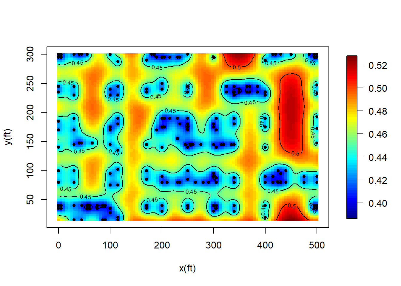

The above ordinary kriging predictor “honors” the data. The predicted surface passes through the data points, i.e., the predicted values at locations where data are measured are identical to the observed values. However, in some situations, we want to predict the less noisy version of data by removing the measurement error. Consider the model \[Y({\mathbf{s}}) = \mu + w({\mathbf{s}}) + \epsilon({\mathbf{s}}).\] We really want to recover the underlying signal \(Z({\mathbf{s}}):=\mu+w({\mathbf{s}})\). To this end, the BLUP is obtained by minimizing \[{\mathbb{E}}(Z({\mathbf{s}}_0)-{\mathbf{a}}^\top {\mathbf{Y}})^2,\ \text{subject to}\ {\mathbf{a}}^\top \mathbf{1} = 1.\] We called it filtered ordinary kriging predictor.

Remark:

i). At unsampled locations, the filtered ordinary kriging predictor is equal to the ordinary kriging predictor. However, at any sampled location, that is \({\mathbf{s}}_1\), …, or \({\mathbf{s}}_n\), filtered ordinary kriging predictor won’t pass the data point, since it removes the white noise \(\epsilon\).

ii). By removing the white noise, the filtered ordinary kriging predictor smooths the data. The larger the variance of \(\sigma_{\epsilon}^2\) is , the more smoothing is the filtered surface.

iii). As we know, the white noise \(\epsilon({\mathbf{s}})\) includes micro-scale variation and measurement errors. In practice, they are usually indistinguishable. So the prediction errors of filtered ordinary kriging predictor don’t include \(\sigma^2_{\epsilon}\). Yet, if the measurement errors are known, say \(\sigma^2_e\), then we should add the micro-scale variance \(\sigma^2_{\epsilon}-\sigma^2_e\) back to the prediction errors of filtered ordinary kriging predictor.

Now we do predictions of C/N ratios at regular grids by removing the noise in Example 3.1.

#Perform filtered ordinary Kriging
s.out <- output.control(signal = TRUE)
pred<-krige.conv(CN.obj, coords=s,locations=sGrid, krige=
krige.control(cov.model="exponential",cov.pars=fit.reml$cov.pars,
nugget=fit.reml$nugget, micro.scale = 0), output=s.out) #plugging theta_{reml}

## krige.conv: model with constant mean
## krige.conv: Kriging performed using global neighbourhood

#Plot the predicted values:
surf <- list()
surf$x <- sx
surf$y <- sy
surf$z <- matrix(pred$predict,nrow = nsx, ncol = nsy)
image.plot(surf, xaxs = "r", yaxs = "r", xlab = "x(ft)",
           ylab = "y(ft)",zlim = range(surf$z))
points(s, pch = 20)
contour(surf, add = T)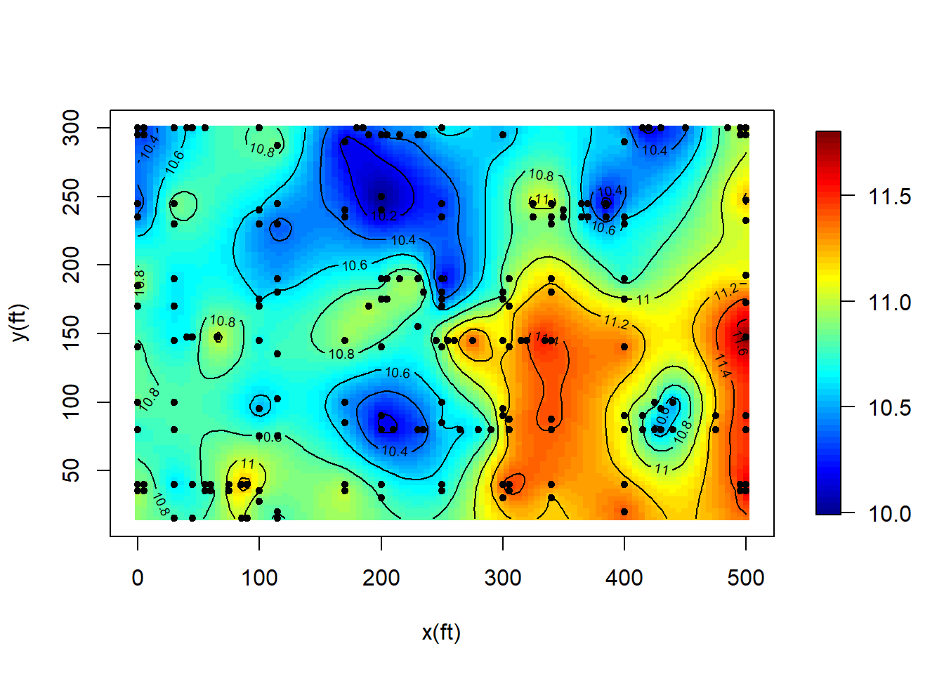

#Plot the standard errors:
surf2 <- surf
surf2$z <- matrix(sqrt(pred$krige.var),nrow = nsx, ncol = nsy)
image.plot(surf2, xaxs = "r",yaxs = "r", xlab = "x(ft)",
           ylab = "y(ft)",zlim = range(surf2$z))
points(s, pch = 20)
contour(surf2, add = T)

3.3 Spatial regression models

In this section, we’ll consider linear regression models for the geostatistical data \(y({\mathbf{s}}_1),..., y({\mathbf{s}}_n)\) with exploratory variables (predictors) \({\mathbf{X}}({\mathbf{s}}_i) = (X_1({\mathbf{s}}_i),X_2({\mathbf{s}}_i),...,X_p({\mathbf{s}}_i))^\top, i=1,2,...,n\). Specifically, at any location \({\mathbf{s}}\in \mathcal{D}\), the response variable \(Y\) is modeled by

\[Y({\mathbf{s}}) = \beta_0 + X_1({\mathbf{s}})\beta_1 + ... + X_p({\mathbf{s}})\beta_p + w({\mathbf{s}}) + e({\mathbf{s}}) = {\mathbf{X}}({\mathbf{s}})^\top {\boldsymbol{\beta}}+ w({\mathbf{s}})+e({\mathbf{s}}),\]

where \({\boldsymbol{\beta}}= (\beta_0,...,\beta_p)^\top\) are unknown coefficients, \(w({\mathbf{s}})\) is a weakly stationary random field with mean zero and covariance function \(C_w({\mathbf{h}})\) and \(e({\mathbf{s}})\) is a white noise with variance \(\sigma_e^2\).

The covariance function of \(Y({\mathbf{s}})\) is \[C_Y({\mathbf{h}}) = \left\{ \begin{array}{ll} C_w({\mathbf{h}}) & \text{if}\ {\mathbf{h}}\neq \mathbf{0}\\ C_w(\mathbf{0}) + \sigma_e^2 & \text{if}\ {\mathbf{h}}= \mathbf{0} \end{array} \right.,\] and the semivariogram of \(Y({\mathbf{s}})\) is \(\gamma_Y({\mathbf{h}}) = C_Y(\mathbf{0}) - C_Y({\mathbf{h}})\). As usual, we’ll use a parametric positive definite function to model \(C_w({\mathbf{h}})\) and hence \(C_Y({\mathbf{h}})\) is also a parametric covariance function, say \(C_Y({\mathbf{h}};{\boldsymbol{\theta}})\), where \({\boldsymbol{\theta}}\) is an unknown vector in \({\mathbb{R}}^q\) including all \(q\) variance and covariance parameters. For example, if we choose the exponential covariance function, that is \(C_w({\mathbf{h}}) = \sigma_w^2 \exp(-||{\mathbf{h}}||/\phi)\), then \({\boldsymbol{\theta}}= (\sigma_w^2, \phi, \sigma_e^2)^\top\) and \(q=3\). In general, Matérn covariance functions are our preferred choices because of the smoothness parameter \(\nu\) characterizing the roughness of the data surface.

Let \({\mathbf{Y}}=(y(s_1), ..., y({\mathbf{s}}_n))^\top\), \(\text{Var}({\mathbf{Y}}) = \Sigma({\boldsymbol{\theta}})\), \[{\mathbf{X}}= \begin{pmatrix} 1 & X_1({\mathbf{s}}_1) &\cdots &X_p({\mathbf{s}}_1)\\ 1& X_1({\mathbf{s}}_2) & \cdots &X_p({\mathbf{s}}_2)\\ \vdots & \vdots & \ddots &\vdots\\ 1& X_1({\mathbf{s}}_n) &\cdots & X_p({\mathbf{s}}_n)\\ \end{pmatrix},\]

and \({\boldsymbol{\epsilon}}= (w({\mathbf{s}}_1)+e({\mathbf{s}}_1), ..., w({\mathbf{s}}_n)+e({\mathbf{s}}_n))^\top\).

Then the data model is \[{\mathbf{Y}}= {\mathbf{X}}{\boldsymbol{\beta}}+ {\boldsymbol{\epsilon}}.\] For model estimations, we are expected to find estimators of the regression coefficients \({\boldsymbol{\beta}}\) and the covariance parameters \({\boldsymbol{\theta}}\). There are still three main methods for estimations, that are variogram methods (classical geostatistical methods), maximum likelihood estimations (MLE) and restricted maximum likelihood (REML) estimations.

We’ll continue the example from Schabenberger and Gotway (2017). In contrast to the analyses in the previous section, we consider the relationship between soil carbon percentage and the soil nitrogen percentage.

Example 3.2 (TC vs. TN) In a study, the total carbon (TC) and total soil nitrogen (TN) percentages were measured at 195 locations on an agriculture fields. One of the research goals is to bulid up a model to study the linear association between TC and TN. The data is included in “CNRatio.csv” and the scatterplot of TC vs. TN is given below.

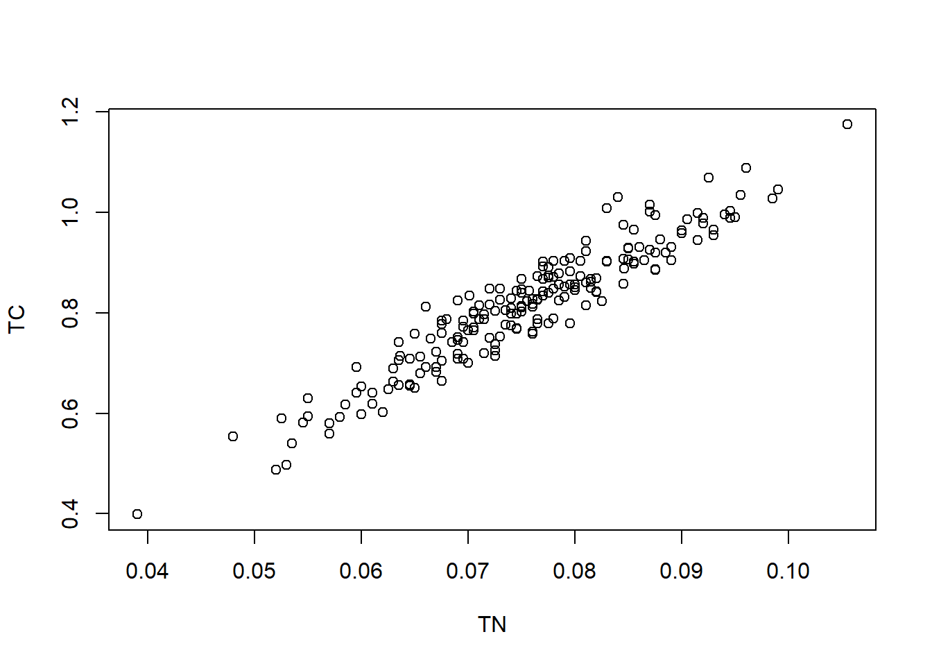
From the above plot, a simple spatial regression model can be considered. Let \(Y({\mathbf{s}})\) be the total carbon at location \({\mathbf{s}}\) and \(X({\mathbf{s}})\) be the total nitrogen at the same location. The model can be written as \[Y({\mathbf{s}}) = \beta_0 + \beta_1 X({\mathbf{s}}) + w({\mathbf{s}}) + e({\mathbf{s}}).\] Again, for simplicity, we use exponential covariance function to model \(C_w({\mathbf{h}})\), which is a special case of Matérn covariance functions.

3.3.1 Spatial estimations

1. Variogram methods

Recall that the Matheron estimator in the previous section. \[\hat \gamma_Y({\mathbf{h}}) = \frac{1}{2|N({\mathbf{h}})|} \sum_{N({\mathbf{h}})}\{y({\mathbf{s}}_i)-y({\mathbf{s}}_j)\}^2.\]

Note that \[\gamma({\mathbf{h}}) = \frac{1}{2}{\text{Var}}(Y({\mathbf{s}}+{\mathbf{h}})-Y({\mathbf{s}})) = \frac{1}{2}{\mathbb{E}}(Y({\mathbf{s}}+{\mathbf{h}})-Y({\mathbf{s}}))^2 - \frac{1}{2}\{{\mathbf{X}}({\mathbf{s}}+{\mathbf{h}})^\top {\boldsymbol{\beta}}-{\mathbf{X}}({\mathbf{s}})^\top{\boldsymbol{\beta}}\}^2.\] The empirical semivariogram such as Matheron estimator cannot be used based on the data \({\mathbf{Y}}\), since the nonconstant mean of \(Y({\mathbf{s}})\) generates bias. Specifically, \[{\mathbb{E}}(\hat \gamma_Y({\mathbf{h}})) = \gamma({\mathbf{h}}) + \frac{1}{2}\{{\mathbf{X}}({\mathbf{s}}+{\mathbf{h}})^\top {\boldsymbol{\beta}}-{\mathbf{X}}({\mathbf{s}})^\top{\boldsymbol{\beta}}\}^2.\] The ideal “data” to construct the empirical semivariogram would be \(Y({\mathbf{s}}_i) - {\mathbf{X}}({\mathbf{s}}_i)^\top {\boldsymbol{\beta}}\). However, we don’t know the values of \({\boldsymbol{\beta}}\) and the BLUE of \({\boldsymbol{\beta}}\), \[ \hat{\boldsymbol{\beta}}_{GLS} = ({\mathbf{X}}^\top \Sigma^{-1}({\boldsymbol{\theta}}){\mathbf{X}})^{-1}{\mathbf{X}}^\top \Sigma^{-1}({\boldsymbol{\theta}}){\mathbf{Y}}, \] depend on the unknown \({\boldsymbol{\theta}}\). Instead, the following iterative algorithm is proposed to estimate \({\boldsymbol{\theta}}\) and \({\boldsymbol{\beta}}\).

i). Use ordinary least squares estimations to obtain an initial estimate of \({\boldsymbol{\beta}}\), say \(\hat {\boldsymbol{\beta}}\);

ii). Compute the residuals \(\hat {\mathbf{e}}= Y({\mathbf{s}}) - {\mathbf{X}}({\mathbf{s}})^\top {\boldsymbol{\beta}}.\) Applying the variogram methods described in Section 3.2, we obtain an estimator of \({\boldsymbol{\theta}}\), say \(\hat {\boldsymbol{\theta}}\).

iii). Plugging \(\hat{\boldsymbol{\theta}}\) to the formula of \(\hat {\boldsymbol{\beta}}_{GLS}\), we obtain a new estimate of \({\boldsymbol{\beta}}\).

iv). Repeat steps ii) and iii) until the relative or absolute change in estimates of \({\boldsymbol{\beta}}\) and \({\boldsymbol{\theta}}\) are small. The relative change criterion means, for estimating an unknown parameter \(\alpha\), the iteration stops when \[\frac{|\hat \alpha_{k+1}-\hat\alpha_{k}|}{0.5(|\hat \alpha_{k+1}|+|\hat\alpha_{k}|)} < 10^{-6},\] where \(\hat \alpha_k\) and \(\hat \alpha_{k+1}\) be the estimators of \(\alpha\) in the \(k\)th and \(k+1\)th iterations.

The above algorithm is termed as iteratively re-weighted generalized least squares (IRWGLS).

Let \({\boldsymbol{\theta}}_{IRWGLS}\) be the final estimator of \({\boldsymbol{\theta}}\). The IRWGLS estimator of \({\boldsymbol{\beta}}\) is

\[ \hat{\boldsymbol{\beta}}_{IRWGLS} = ({\mathbf{X}}^\top \Sigma^{-1}({\boldsymbol{\theta}}_{IRWGLS}){\mathbf{X}})^{-1}{\mathbf{X}}^\top \Sigma^{-1}({\boldsymbol{\theta}}_{IRWGLS}){\mathbf{Y}}, \]

and its variance can be estimated as

\[ {\text{Var}}(\hat{\boldsymbol{\beta}}_{IRWGLS})\approx ({\mathbf{X}}^\top \Sigma^{-1}({\boldsymbol{\theta}}_{IRWGLS}){\mathbf{X}})^{-1}.\]

Remark: The bias problem in constructing the empirical semivariogram is not fully solved by the IRWGLS algorithm.

2. Maximum likelihood estimations (MLE)

In contrast to the IRWGLS approach, MLE are simultaneous estimations of mean and covariance parameters. Assume that \(Y({\mathbf{s}})\) is a Gaussian random field. We can apply the MLE method in Section 2.4 to estimate \({\boldsymbol{\theta}}\) and \({\boldsymbol{\beta}}\), which can be obtained by maximizing the following log likelihood function \[\log \ell({\boldsymbol{\beta}},{\boldsymbol{\theta}}; {\mathbf{Y}}) = -\frac{n}{2}\log(2\pi)-\frac{1}{2}\log|\Sigma({\boldsymbol{\theta}})| - \frac{1}{2}({\mathbf{Y}}-{\mathbf{X}}{\boldsymbol{\beta}})^\top \Sigma^{-1}({\boldsymbol{\theta}})({\mathbf{Y}}-{\mathbf{X}}{\boldsymbol{\beta}}).\] Let \(\hat {\boldsymbol{\beta}}_{ml}\) and \(\hat {\boldsymbol{\theta}}_{ml}\) be the MLE of \({\boldsymbol{\beta}}\) and \({\boldsymbol{\theta}}\) respectively. Their variance-covariance matrix can be estimated based on fisher information matrix. Specifically, the variance of \(\hat {\boldsymbol{\beta}}_{ml}\) is \[ {\text{Var}}(\hat{\boldsymbol{\beta}}_{ml})\approx ({\mathbf{X}}^\top \Sigma^{-1}({\boldsymbol{\theta}}_{ml}){\mathbf{X}})^{-1}.\] and the variance of \(\hat {\boldsymbol{\theta}}_{ml}\) is \[ {\text{Var}}(\hat{\boldsymbol{\theta}}_{ml})\approx B(\hat {\boldsymbol{\theta}}_{ml})^{-1},\] where \(B({\boldsymbol{\theta}})\) is a \(q\times q\) matrix whose \((i,j)\)th element is \[\frac{1}{2}\text{tr}\left(\Sigma^{-1}({\boldsymbol{\theta}})\frac{\partial{\Sigma({\boldsymbol{\theta}})}}{\partial{\theta_i}}\Sigma^{-1}({\boldsymbol{\theta}})\frac{\partial{\Sigma({\boldsymbol{\theta}})}}{\partial{\theta_j}}\right).\]

3. Restricted maximum likelihood estimations (REML)

In Section 3.2, we’ve derived REML estimations for spatial regression models and specify the error contrasts matrix \(K\) when the mean function is constant. Here, we provide a representation of the likelihood by eliminating the matrix \(K\) from the expression.

Suppose that the rank of \({\mathbf{X}}\) is \(k\). Then, the log likelihood function of \(K{\mathbf{Y}}\) is \[ \begin{align*} &\log \ell({\boldsymbol{\theta}}; {\mathbf{Y}}) = -\frac{n-k}{2}\log(2\pi)-\frac{1}{2}\log|K\Sigma({\boldsymbol{\theta}})K^\top| - \frac{1}{2}{\mathbf{Y}}^\top K^\top \Sigma^{-1}({\boldsymbol{\theta}})K{\mathbf{Y}}\\ =& -0.5(n-k)\log(2\pi)-0.5\log|\Sigma({\boldsymbol{\theta}})| - 0.5\log|{\mathbf{X}}^\top \Sigma({\boldsymbol{\theta}})^{-1}{\mathbf{X}}| +0.5\log{|{\mathbf{X}}^\top {\mathbf{X}}|}-0.5{\mathbf{r}}^\top \Sigma({\boldsymbol{\theta}})^{-1}{\mathbf{r}}, \end{align*} \] where \[{\mathbf{r}}= {\mathbf{Y}}- ({\mathbf{X}}^\top \Sigma({\boldsymbol{\theta}})^{-1}{\mathbf{X}})^{-1}{\mathbf{X}}^\top \Sigma({\boldsymbol{\theta}})^{-1}{\mathbf{Y}}.\]

Let \(\hat{\boldsymbol{\theta}}_{reml}\) be the REML estimators. The mean \({\boldsymbol{\beta}}\) can be obtained by

\[({\mathbf{X}}^\top \Sigma^{-1}(\hat{\boldsymbol{\theta}}_{reml}){\mathbf{X}})^{-1}{\mathbf{X}}^\top \Sigma^{-1}(\hat{\boldsymbol{\theta}}_{reml}){\mathbf{Y}}.\]

3.3.2 Spatial prediction (Kriging)

Recall that \[Y({\mathbf{s}}) = {\mathbf{X}}({\mathbf{s}})^\top{\boldsymbol{\beta}}+ w({\mathbf{s}}) + e({\mathbf{s}}).\] Unlike Section 3.2, the mean function here is a linear function. The prediction method for the above spatial regression model is called universal kriging, which is also the best linear unbiased prediction.

Let \[{\mathbf{c}}({\boldsymbol{\theta}})={\text{Cov}}({\mathbf{Y}}, Y({\mathbf{s}}_0)) = (C_Y({\mathbf{s}}_1-{\mathbf{s}}_0;{\boldsymbol{\theta}}),...,C_Y({\mathbf{s}}_n-{\mathbf{s}}_0;{\boldsymbol{\theta}}))^\top,\] and let \[\Sigma({\boldsymbol{\theta}}) = {\text{Var}}({\mathbf{Y}}) = (C_Y({\mathbf{s}}_i-{\mathbf{s}}_j;{\boldsymbol{\theta}}))_{i,j=1}^n.\] Note that both \({\mathbf{c}}({\boldsymbol{\theta}})\) and \(\Sigma({\boldsymbol{\theta}})\) depends on the unknown \({\boldsymbol{\theta}}\), the parameters of the covariance function. Following the similar proof in Chapter \(1\) Example 1.5, we can derive the BLUP of \(Y\) at location \({\mathbf{s}}_0\) can be written as, \[\hat Y({\mathbf{s}}_0) = {\mathbf{X}}({\mathbf{s}}_0)^\top \hat {\boldsymbol{\beta}}_{gls} + {\mathbf{c}}({\boldsymbol{\theta}})^\top\Sigma({\boldsymbol{\theta}})^{-1}({\mathbf{Y}}-{\mathbf{X}}\hat {\boldsymbol{\beta}}_{gls}),\] where \[\hat {\boldsymbol{\beta}}_{gls}= ({\mathbf{X}}^\top \Sigma({\boldsymbol{\theta}})^{-1}{\mathbf{X}})^{-1}({\mathbf{X}}^\top \Sigma({\boldsymbol{\theta}})^{-1}{\mathbf{Y}}).\] The variance of \(\hat Y({\mathbf{s}}_0)\) is \[ \begin{align*} {\text{Var}}(\hat Y({\mathbf{s}}_0)) &= C_Y(\mathbf{0}) - {\mathbf{c}}({\boldsymbol{\theta}})^\top \Sigma({\boldsymbol{\theta}})^{-1}{\mathbf{c}}({\boldsymbol{\theta}})\\ &+ ({\mathbf{X}}({\mathbf{s}}_0)^\top - {\mathbf{c}}({\boldsymbol{\theta}})^\top \Sigma({\boldsymbol{\theta}})^{-1}{\mathbf{X}})({\mathbf{X}}^\top \Sigma({\boldsymbol{\theta}})^{-1}{\mathbf{X}})^{-1}({\mathbf{X}}({\mathbf{s}}_0)^\top - {\mathbf{c}}({\boldsymbol{\theta}})^\top \Sigma({\boldsymbol{\theta}})^{-1}{\mathbf{X}})^\top. \end{align*} \] To get the prediction, we have to substitute \({\boldsymbol{\theta}}\) with its estimator \(\hat {\boldsymbol{\theta}}\), which can be obtained by variogram methods, ML or REML estimations. Eventually, we get the estimated BLUP, so-called EBLUP.

3.3.3 Inference and Model comparisons

In this section, we’ll introduce how to do hypothesis testing and how to construct confidence intervals for the parameters \({\boldsymbol{\beta}}\) and \({\boldsymbol{\theta}}\). Then, we discuss some problems on model comparisons.

According to the estimation procedures introduced in Section 3.3.1, we know that \({\boldsymbol{\beta}}\) is estimated by an EGLS estimator, that is \[\hat {\boldsymbol{\beta}}= ({\mathbf{X}}^\top \Sigma^{-1}(\hat{\boldsymbol{\theta}}){\mathbf{X}})^{-1}{\mathbf{X}}^\top \Sigma^{-1}(\hat{\boldsymbol{\theta}}){\mathbf{Y}},\] where \(\hat {\boldsymbol{\theta}}\) can be either the IRWGLS, ML or REML estimators.

Under some regularity conditions (see details in Schabenberger and Gotway (2017)), \(\hat {\boldsymbol{\beta}}\) asymptotically follows Gaussian distribution. Specifically, \[\hat {\boldsymbol{\beta}}\sim Gaussian({\boldsymbol{\beta}}, ({\mathbf{X}}^\top \Sigma^{-1}({\boldsymbol{\theta}}){\mathbf{X}})^{-1}).\] Since \({\boldsymbol{\theta}}\) is unknown, it is usually replaced by \(\hat {\boldsymbol{\theta}}\), which of course may make the probability of type I error not be well controlled in a hypothesis testing.

1. Hypothesis testing about fixed effects. Let \(A\) be a \(m\times (p+1)\) matrix and \(a\) be a \(m\times 1\) vector. In applications, many hypothesis testings regarding \({\boldsymbol{\beta}}\) can be written as \[H_0: \ A{\boldsymbol{\beta}}= {\mathbf{a}}\ vs.\ H_a: \ A{\boldsymbol{\beta}}\neq {\mathbf{a}}.\] Here are some examples.

i). If we want to test \(H_0: \beta_2 = 0\ vs.\ H_a: \beta_2\neq 0\), then \(m=1\), \({\mathbf{a}}=0\) and \(A=(0,0, 1,0,..,0)\);

ii). If we want to test \(H_0: \beta_1 = ... = \beta_p = 0,\ vs.\ H_a: \ \text{at least one of}\ \beta_i,i=1,...,p \ \text{is nonzero}\), then \(m=p\), \({\mathbf{a}}=(0,0,...,0)^\top\), and \(A\) is \(p\times (p+1)\) matrix given by \[A = \begin{pmatrix} 0 & 1 & 0 &\cdots &0\\ 0 & 0 & 1 &\cdots & 0\\ \vdots & \vdots & \ddots &\ddots& \vdots\\ 0 & 0 &\cdots & 0&1\\ \end{pmatrix};\]

iii). If we want to test \(H_0: \beta_1 =\beta_2,\ vs. \ H_a: \beta_1 \neq \beta_2\), then \(m=1\), \({\mathbf{a}}=0\), and \(A = (0, 1, -1, 0, ..., 0)\).

Define the Wald F statistic \[ F = \frac{(A\hat{\boldsymbol{\beta}}- {\mathbf{a}})^\top\{A({\mathbf{X}}^\top \Sigma(\hat {\boldsymbol{\theta}})^{-1}{\mathbf{X}})^{-1}A^\top\}^{-1}(A\hat{\boldsymbol{\beta}}- {\mathbf{a}})}{rank(A)}.\] When \(\hat {\boldsymbol{\theta}}\) is consistent, i.e., \(\hat {\boldsymbol{\theta}}\) converges to \({\boldsymbol{\theta}}\) in probability as sample size \(n\to \infty\), \(F\) can be approximated by a F distribution with \(rank(A)\) numerator and \(n-rank({\mathbf{X}})\) denominator degrees of freedom.

Hence, given a significance level \(\alpha\), \(H_0\) is rejected when \(F > F_{\alpha, rank(A), n-rank(X)}\).

Example 3.3 (Single coefficient inference) Consider the test \(H_0: \beta_2 = 0\ vs.\ H_a: \beta_2\neq 0\). The F statistic can be reduced to t-test. Let \(s_{22}\) be the \((2,2)\)th element of \(({\mathbf{X}}^\top \Sigma(\hat {\boldsymbol{\theta}})^{-1}{\mathbf{X}})^{-1}\). Then \(H_0\) is rejected when \(|\hat \beta_{2}|/\sqrt{s_{22}} > t_{\alpha/2,n-rank({\mathbf{X}})}\). And the \(100(1-\alpha)\)% confidence interval for \(\beta_2\) is \[\hat \beta_2 \pm \sqrt{s_{22}}t_{\alpha/2,n-rank({\mathbf{X}})},\] where \(t_{\alpha/2,n-rank({\mathbf{X}})}\) is the \(100(1-\alpha/2)\)th percentile of a \(t\)-distribution with degrees of freedom \(n-rank({\mathbf{X}})\).

2. Hypothesis testings about covariance parameters. The distribution property of \(\hat \theta_{IRWGLS}\) is unclear. Hence, the inference on covariance parameters \({\boldsymbol{\theta}}\) is based either on the ML or on the REML estimators, which asymptotically follows Gaussian distribution. The approximate confidence intervals or associated hypothesis tests (\(H_0: \theta_i = 0\ vs.\ H_a: \theta_i \neq 0\)) can be obtained using \[\hat \theta_{i,ml} \pm z_{\alpha/2}\sqrt{{\text{Var}}(\hat \theta_{i,ml})},\] or \[\hat \theta_{i,reml} \pm z_{\alpha/2}\sqrt{{\text{Var}}(\hat \theta_{i,reml})},\] where \(z_{\alpha/2}\) is the \(100(1-\alpha/2)\)th percentile of standard normal distribution, and the variance of the estimators (\({\text{Var}}(\hat \theta_{i})\)) derives from the inverse of expected fisher information matrix. Refer to Section 3.3.1 for the form of \({\text{Var}}(\hat \theta_{i,ml})\).

3. Model comparisons. Sometimes we are interested in comparing two nested models (full model vs reduced model) to see whether a subset of parameters fits the data as well as the full set. Here are some examples.

Example 3.4 (model comparisons) Consider the following spatial regression model: \[Y({\mathbf{s}}) = \beta_0 + \beta_1X_1({\mathbf{s}}) + w({\mathbf{s}}) +e({\mathbf{s}}),\] where the covariance function of \(Y\) is modeled by exponential covariance function with nugget effect, that is \[C_Y({\mathbf{h}}) = \left\{ \begin{array}{ll} \sigma_w^2 \exp(-||{\mathbf{h}}||/\phi) & \text{if}\ {\mathbf{h}}\neq \mathbf{0}\\ \sigma_w^2 + \sigma_e^2 & \text{if}\ {\mathbf{h}}= \mathbf{0} \end{array} \right.\]

i). If we want to see whether there is nugget effect in the model, we need to compare the full model \[Y({\mathbf{s}}) = \beta_0 + \beta_1X_1({\mathbf{s}}) + w({\mathbf{s}}) +e({\mathbf{s}})\] with the reduced model \[Y({\mathbf{s}}) = \beta_0 + \beta_1X_1({\mathbf{s}}) + w({\mathbf{s}}).\] To this end, we can consider the test \[H_0: \sigma_e^2 = 0 \ vs. \ H_a: \sigma_e^2 > 0.\]

ii). If we want to see whether the predictor \(X_1\) is useful, we need to compare the full model \[Y({\mathbf{s}}) = \beta_0 + \beta_1X_1({\mathbf{s}}) + w({\mathbf{s}}) +e({\mathbf{s}})\] with the reduced model \[Y({\mathbf{s}}) = \beta_0 + w({\mathbf{s}}) +e({\mathbf{s}}).\] To this end, we can consider the test \[H_0: \beta_1= 0 \ vs. \ H_a: \beta_1 \neq 0.\]

The model comparison problems above can be solved by the F test and z test introduced in part1&2. Yet, there is an alternative method called likelihood ratio test.

Consider two models of the same form (nested models), one based on parameter \({\boldsymbol{\theta}}_1\) and a larger model based on \({\boldsymbol{\theta}}_2\), with \(dim({\boldsymbol{\theta}}_2) > dim({\boldsymbol{\theta}}_1)\). That is, \({\boldsymbol{\theta}}_1\) is obtained by constraining some parameters in \({\boldsymbol{\theta}}_2\), usually setting them to zero and \(dim({\boldsymbol{\theta}})\) denotes the number of free parameters. Model comparison is reduced to consider the test \[H_0: {\boldsymbol{\theta}}= {\boldsymbol{\theta}}_1 \ vs.\ H_a: {\boldsymbol{\theta}}= {\boldsymbol{\theta}}_2.\] Let \(\phi({\boldsymbol{\beta}};{\mathbf{Y}})\) be twice the negative of log-likelihood. The likelihood ratio statistic is defined by \[LR = \phi({\boldsymbol{\theta}}_1;{\mathbf{Y}}) - \phi({\boldsymbol{\theta}}_2;{\mathbf{Y}}),\] which asymptotically follows a \(\chi^2\) distribution with degrees of freedom \(dim({\boldsymbol{\theta}}_2)-dim({\boldsymbol{\theta}}_1)\).

So \(H_0\) is rejected when \(LR > \chi^2_{\alpha,dim({\boldsymbol{\theta}}_2)-dim(\theta_1)}\) or the p-value is less than \(\alpha\), where \(\chi^2_{\alpha,dim({\boldsymbol{\theta}}_2)-dim(\theta_1)}\) is the \(100(1-\alpha)\)th percentile of a \(\chi^2\) distribution with degrees of freedom \(dim({\boldsymbol{\theta}}_2)-dim({\boldsymbol{\theta}}_1)\). There is an important exception. If we set some parameter to the boundary of parameter space, for example, the test of \(H_0: \sigma_e^2 = 0\), then we should use the threshold \(\chi^2_{2\alpha,dim({\boldsymbol{\theta}}_2)-dim(\theta_1)}\) or divide the p-value derived from a \(\chi^2\) distribution with degrees of freedom \(dim({\boldsymbol{\theta}}_2)-dim({\boldsymbol{\theta}}_1)\) by 2.

Example 3.5 (test of spatial dependence of TC) If we want to know whether there exists spatial dependence after doing regression of the total carbon (TC) percentages on the total soil nitrogen (TN) percentages, we could consider compare the following two models \[Y({\mathbf{s}}) = \beta_0 + \beta_1X_1({\mathbf{s}}) + e({\mathbf{s}}),\ \text{with}\ \text{Cov}(e({\mathbf{s}}_i),e({\mathbf{s}}_j))=\sigma^2\exp(-||{\mathbf{s}}_i-{\mathbf{s}}_j||/\phi)\] and \[Y({\mathbf{s}}) = \beta_0 + \beta_1X_1({\mathbf{s}}) + e({\mathbf{s}}),\ \text{with}\ \text{Cov}(e({\mathbf{s}}_i),e({\mathbf{s}}_j))=\sigma^2 \mathbf{1}_{\{i=j\}}.\] When \(\phi \to 0\), the model with spatial dependence approaches the independence model. If we reparameterize the covariance model by letting \[\theta = \exp(-1/\phi),\] then the model comparison is reduced to test \($H_0: \theta = 0\ vs. \ H_a: \theta >0\). Applying likelihood ratio test, we reject \(H_0\) if the p-value is small.

Sometimes, the models we want to compare are not nested (\({\boldsymbol{\theta}}_1\) is not a subset of \({\boldsymbol{\theta}}_2\)). In this case, we can use AIC or BIC to do model comparison. AIC is given by \[AIC = \phi({\boldsymbol{\theta}};{\mathbf{Y}}) + 2dim({\boldsymbol{\theta}}),\] and BIC is given by \[BIC = \phi({\boldsymbol{\theta}};{\mathbf{Y}}) + dim({\boldsymbol{\theta}})\log n.\]

Now we are ready to do estimation and inference for Example 3.2.

rm(list=ls())
library(geoR)
library(spBayes)
dat <- read.csv("./data/CNRatio.csv", header = TRUE)
s <- dat[,1:2]#coordinates
ns <- nrow(s)
TN <- dat[,3]#TN
TC <- dat[,4]#TC

#training and testing sets
set.seed(1)
sIndx <- sample(1:ns, 0.8*ns)
s.train <- s[sIndx, ]
s.test <- s[-sIndx, ]
TN.train <- TN[sIndx]
TN.test <- TN[-sIndx]
TC.train <- TC[sIndx]
TC.test <- TC[-sIndx]
plot(s.train)
points(s.test, col ="red")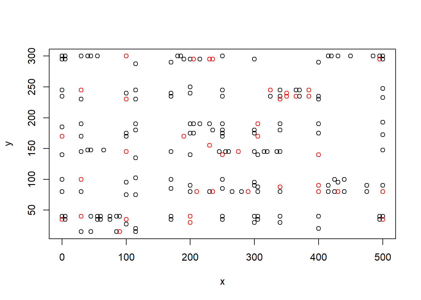

max.dist <-  0.5 * max(iDist(s.train))

plot(TN.train, TC.train, xlab = "TN", ylab = "TC")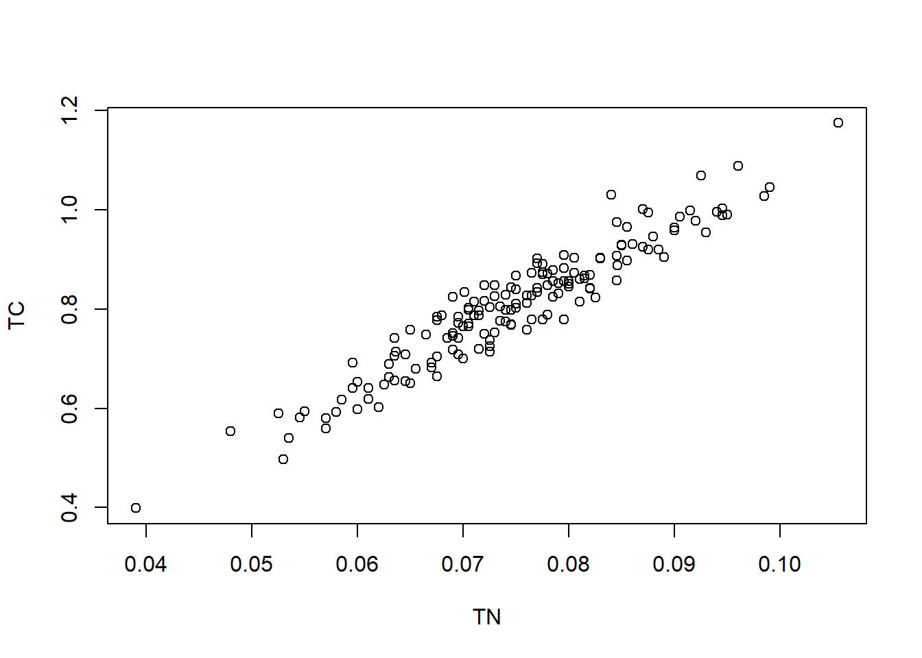

m1 <- lm(TC.train~TN.train)
m1.sum <- summary(m1)

bins <- 100
#Matheron estimator
vario.M <- variog(coords = s.train, data = TC.train, trend = ~TN.train,
                  estimator.type = "classical", uvec = (seq(0, max.dist, l = bins )))

## variog: computing omnidirectional variogram

#Cressie-Hawkins estimator
vario.CH <- variog(coords = s.train, data = TC.train, trend = ~TN.train,
                   estimator.type = "modulus", uvec = (seq(0, max.dist, l = bins )))

## variog: computing omnidirectional variogram

plot(vario.M, main = "TC")
points(vario.CH$u, vario.CH$v, col = "red")
legend("bottomright", legend=c("Matheron", "Cressie-Hawkins"), pch = c(1,1),
       col = c("black", "red"), cex = 0.6)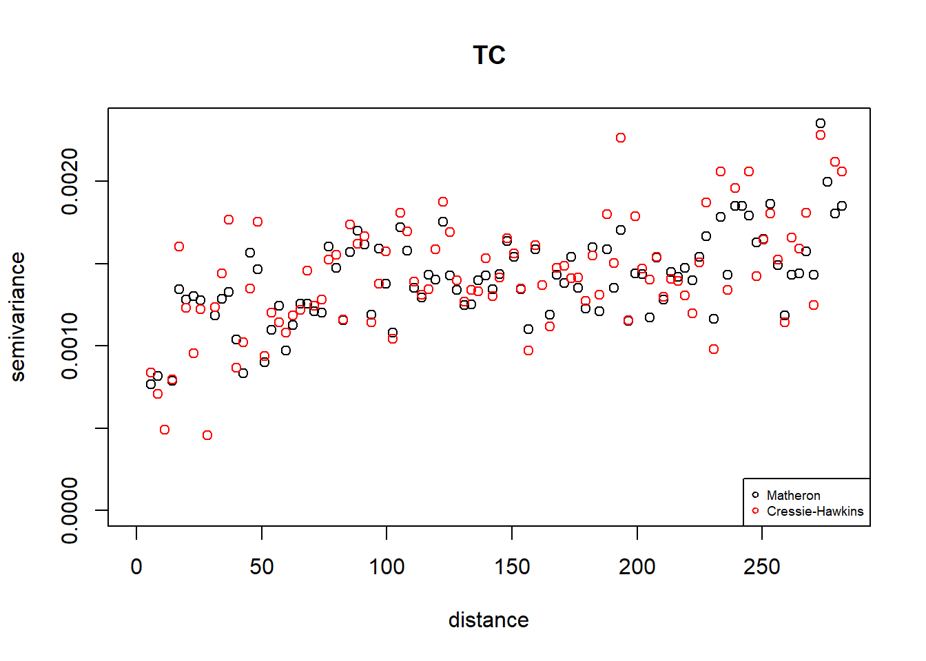

#WLS with weights N(h)/gamma^2(h)
fit.vario <- variofit(vario.M, ini.cov.pars = c(m1.sum$sigma^2, -max.dist/log(0.05)),
         cov.model = "exponential", minimisation.function = "optim", weights = "cressie",
         control = list(factr=1e-10, maxit = 500), messages = FALSE)

fit.vario

## variofit: model parameters estimated by WLS (weighted least squares):
## covariance model is: exponential
## parameter estimates:
##   tausq sigmasq     phi 
##  0.0000  0.0030 94.0605 
## Practical Range with cor=0.05 for asymptotic range: 281.7801
## 
## variofit: minimised weighted sum of squares = 2123.161

#MLE
fit.ml<- likfit(coords = s.train, data = TC.train, trend =~TN.train, ini.cov.pars =
                    c(m1.sum$sigma^2, -max.dist/log(0.05)), cov.model = "exponential",
                  lik.method = "ML", control = list(factr=1e-10, maxit = 500))

## kappa not used for the exponential correlation function
## ---------------------------------------------------------------
## likfit: likelihood maximisation using the function optim.
## likfit: Use control() to pass additional
##          arguments for the maximisation function.
##         For further details see documentation for optim.
## likfit: It is highly advisable to run this function several
##         times with different initial values for the parameters.
## likfit: WARNING: This step can be time demanding!
## ---------------------------------------------------------------
## likfit: end of numerical maximisation.

fit.ml

## likfit: estimated model parameters:
##     beta0     beta1     tausq   sigmasq       phi 
## " 0.0009" "10.8093" " 0.0005" " 0.0010" "41.9629" 
## Practical Range with cor=0.05 for asymptotic range: 125.7095
## 
## likfit: maximised log-likelihood = 307.8

#REML
fit.reml<- likfit(coords = s.train, data = TC.train, trend =~TN.train, ini.cov.pars =
                  c(m1.sum$sigma^2, -max.dist/log(0.05)), cov.model = "exponential",
                lik.method = "REML", control = list(factr=1e-10, maxit = 500))

## kappa not used for the exponential correlation function
## ---------------------------------------------------------------
## likfit: likelihood maximisation using the function optim.
## likfit: Use control() to pass additional
##          arguments for the maximisation function.
##         For further details see documentation for optim.
## likfit: It is highly advisable to run this function several
##         times with different initial values for the parameters.
## likfit: WARNING: This step can be time demanding!
## ---------------------------------------------------------------
## likfit: end of numerical maximisation.

fit.reml

## likfit: estimated model parameters:
##     beta0     beta1     tausq   sigmasq       phi 
## " 0.0011" "10.8120" " 0.0005" " 0.0011" "49.2419" 
## Practical Range with cor=0.05 for asymptotic range: 147.5154
## 
## likfit: maximised log-likelihood = 304.2

#compare TN.test with pred$predict#prediction at s.test
TC.train.obj <- as.geodata(cbind(s.train, TC.train, TN.train), coords.col = 1:2,
                     data.col = 3, covar.col = 4)
TC.test.obj <- as.geodata(cbind(s.test, TC.test, TN.test),
                     coords.col = 1:2, data.col = 3, covar.col = 4)
#Perform universal Kriging
pred<-krige.conv(TC.train.obj,locations=s.test, krige=
                 krige.control(type.krige = "OK", obj.model = fit.ml,
                trend.d = trend.spatial(~TN.train, geodata = TC.train.obj),
                trend.l = trend.spatial(~TN.test,geodata = TC.test.obj)))

## krige.conv: model with covariates matrix provided by the user
## krige.conv: Kriging performed using global neighbourhood

plot(TC.test, pred$predict)
abline(a= 0,b = 1)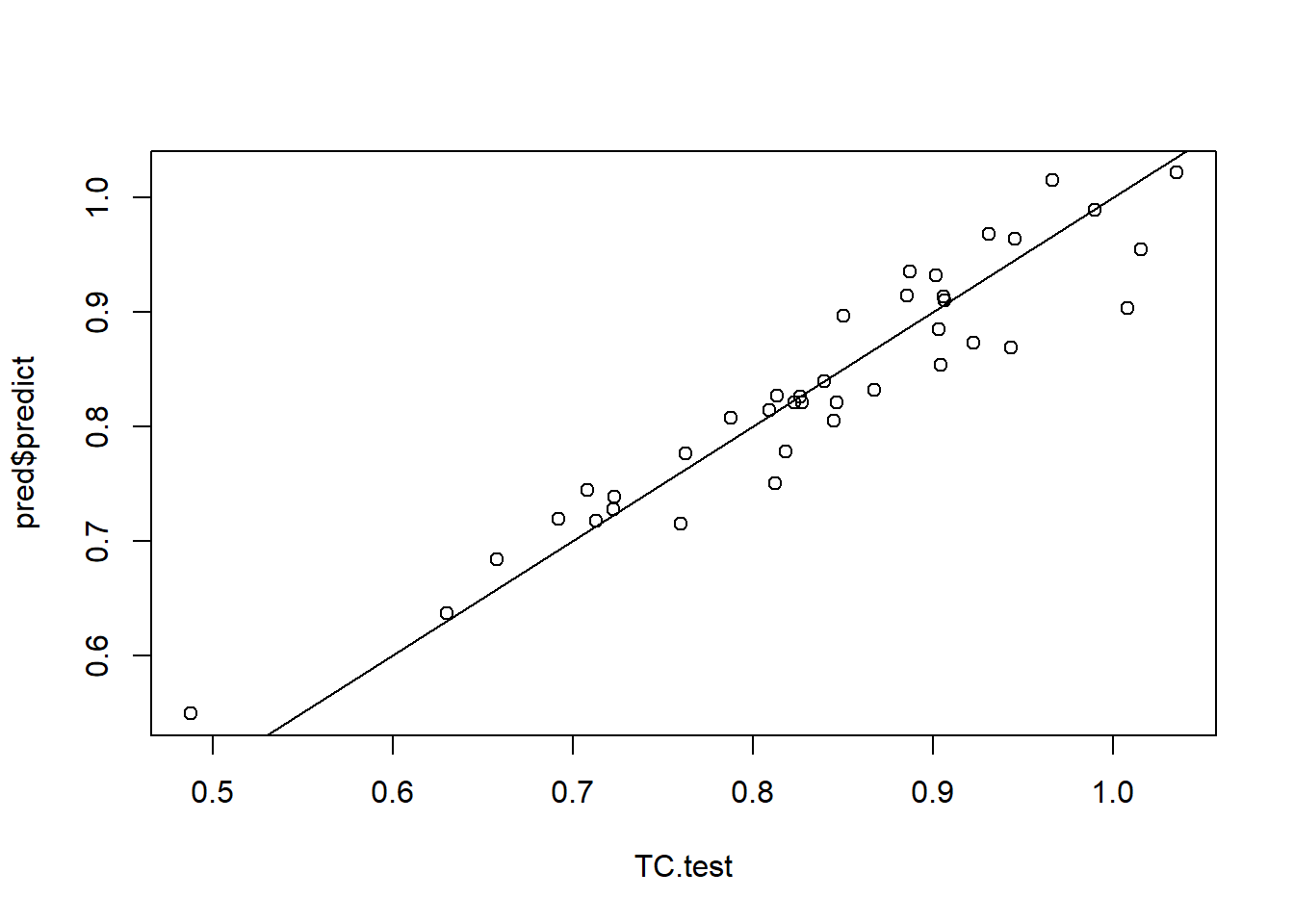

#plot prediction standard errors
plot(sqrt(pred$krige.var))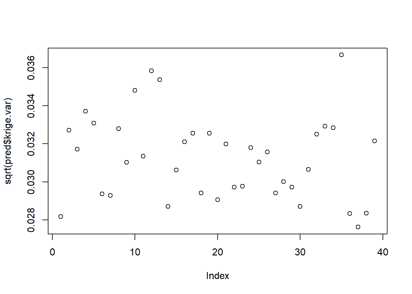

#test the linear association between TN and TC: H_0: \beta_1 = 0 vs Ha: beta_1 \neq = 0
#95% CI for \beta_1
beta1.hat <- fit.ml$beta[[2]]
ME <- sqrt(fit.ml$beta.var[2,2])*qt(1-0.05/2, nrow(s.train)-2)
CI <- c(beta1.hat-ME, beta1.hat + ME)
CI

## [1] 10.16402 11.45453

#test whether there is nugget effect: H_0: \sigma_e^2 = 0 vs. H_a: \sigma_e^2 > 0
fit.ml.noNug <- likfit(coords = s.train, data = TC.train, trend =~TN.train, ini.cov.pars =
                       c(m1.sum$sigma^2, -max.dist/log(0.05)), fix.nugget = TRUE,
                       nugget = 0, cov.model = "exponential",lik.method = "ML")

## kappa not used for the exponential correlation function
## ---------------------------------------------------------------
## likfit: likelihood maximisation using the function optimize.
## likfit: Use control() to pass additional
##          arguments for the maximisation function.
##         For further details see documentation for optimize.
## likfit: It is highly advisable to run this function several
##         times with different initial values for the parameters.
## likfit: WARNING: This step can be time demanding!
## ---------------------------------------------------------------
## likfit: end of numerical maximisation.

fit.ml.noNug

## likfit: estimated model parameters:
##     beta0     beta1   sigmasq       phi 
## " 0.0010" "10.7819" " 0.0016" "14.7937" 
## Practical Range with cor=0.05 for asymptotic range: 44.31802
## 
## likfit: maximised log-likelihood = 303.6

#p-value of likelihood ratio test
LR.obs <- -2 * (fit.ml.noNug$loglik - fit.ml$loglik)
p.value <- 0.5*(1-pchisq(LR.obs, 1))
p.value

## [1] 0.001907926

#test of spatial dependence of TC.
LR <- -2 *(fit.ml.noNug$nospatial$loglik.ns - fit.ml.noNug$loglik)
p.value <- 0.5*(1-pchisq(LR.obs, 1))
p.value

## [1] 0.001907926

3.4 Spatial generalized linear mixed model for non-Gaussian data

So far, the spatial random field \(Y({\mathbf{s}})\) is assumed to take values in the real line \((-\infty, \infty)\), which is a continuous variable. Moreover, most of time we assume it is Gaussian random field. However,

1. what if the distribution of data is highly skewed?

2. what if the data have bounded support such as proportions?

3. what if the data only take discrete values, such as spatial count data, binary data?

If the spatial data are continuous, one possibility is to transform them to be close to Gaussian distribution. For example, we can use Box-Cox transformations. However, it does not always work. In general, we need borrow the modeling ideas of classical generalized linear mixed models (GLMM).

Recall that the modeling framework we used in the previous sections,

\[Y({\mathbf{s}}) = {\mathbf{X}}({\mathbf{s}})^\top {\boldsymbol{\beta}}+ w({\mathbf{s}}) + e({\mathbf{s}}).\] Within this framework, the random field is simply a summation of its linear mean function and variance process (spatial variability and measurement errors). For non-Gaussian data, it doesn’t work. For example, if \(Y\) is a binary spatial random field, that is \(Y\) only takes value \(0\) or \(1\), \({\mathbf{X}}({\mathbf{s}})^\top {\boldsymbol{\beta}}\) is not an appropriate mean function and the residuals obtained by taking the difference of \(Y\) and its mean are not appropriate to be modeled as a continuous spatial random field.

In order to introduce models for non-Gaussian spatial data, let’s go beyond the additive modeling ideas, which usually decompose the response variables by its means and variance components. An alternative way to generate statistical models is hierarchical modeling, which usually involves conditional distributions.

With this new perspective, the original additive Gaussian spatial regression model (\(Y({\mathbf{s}}) = {\mathbf{X}}({\mathbf{s}})^\top {\boldsymbol{\beta}}+ w({\mathbf{s}}) + e({\mathbf{s}})\)) can be equivalently specified as

\[ \begin{align*} &Y({\mathbf{s}}) | \mu({\mathbf{s}}) \stackrel{ind.}{\sim} Gaussian(\mu({\mathbf{s}}), \sigma_e^2),\\ &\mu({\mathbf{s}}) \sim Gaussian({\mathbf{X}}({\mathbf{s}})^\top {\boldsymbol{\beta}}, C_w({\mathbf{h}})). \end{align*} \] Now we can easily generalize the above hierarchical model to non-Gaussian spatial data. The resulting model is called spatial generalized linear mixed model (SGLMM), which was first introduced by P. J. Diggle, Tawn, and Moyeed (1998).

Example 3.6 Assume that the response variable \(Y\) is a binary spatial random field and \({\mathbf{X}}=(X_1,...,X_p)\) are predictors. We can model the spatial dependence of \(Y\) and the relationshiop between \(Y\) and \({\mathbf{X}}\) via the following SGLMM. \[ \begin{align*} &Y({\mathbf{s}}) | \pi({\mathbf{s}}) \stackrel{ind.}{\sim} Bernoulli(\pi({\mathbf{s}}))\\ &logit(\pi({\mathbf{s}})) \sim Gaussian({\mathbf{X}}({\mathbf{s}})^\top {\boldsymbol{\beta}}, C({\mathbf{h}};{\boldsymbol{\theta}})), \end{align*} \] where \(logit(\pi) := \log(\pi/(1-\pi))\) and \(C({\mathbf{h}})\) is a weakly stationary covariance function.

The distribution of \(Bernoulli(\pi)\) is given by \[f_Y(k) = \pi^k (1-\pi)^{1-k}, k = 0, 1.\]

Example 3.7 Assume that the response variable \(Y\) is spatial count random field whose distribution at location \({\mathbf{s}}\) follows Poisson distribution and \({\mathbf{X}}=(X_1,...,X_p)\) are predictors. We can model the spatial dependence of \(Y\) and the relationshiop between \(Y\) and \({\mathbf{X}}\) via the following SGLMM. \[ \begin{align*} &Y({\mathbf{s}}) | \lambda({\mathbf{s}}) \stackrel{ind.}{\sim} Poisson(\lambda({\mathbf{s}}))\\ &log(\lambda({\mathbf{s}})) \sim Gaussian({\mathbf{X}}({\mathbf{s}})^\top {\boldsymbol{\beta}}, C({\mathbf{h}};{\boldsymbol{\theta}})), \end{align*} \] where \(C({\mathbf{h}})\) is a weakly stationary covariance function.

The distribution of \(Poisson(\lambda)\) is given by \[f_Y(k) = \frac{e^{-\lambda}\lambda^k}{k!}, k=0,1,...\]

Example 3.8 Assume that the response variable \(Y\) is countinous spatial random field whose distribution at location \({\mathbf{s}}\) follows Gamma distribution and \({\mathbf{X}}=(X_1,...,X_p)\) are predictors. We can model the spatial dependence of \(Y\) and the relationshiop between \(Y\) and \({\mathbf{X}}\) via the following SGLMM. \[ \begin{align*} &Y({\mathbf{s}}) | \mu({\mathbf{s}}) \stackrel{ind.}{\sim} Gamma(\mu({\mathbf{s}}), \nu)\\ &\log(\mu({\mathbf{s}})) \sim Gaussian({\mathbf{X}}({\mathbf{s}})^\top {\boldsymbol{\beta}}, C({\mathbf{h}};{\boldsymbol{\theta}})), \end{align*} \] where \(C({\mathbf{h}})\) is a weakly stationary covariance function.

The density of \(Gamma(\mu,\nu)\) is given by \[f_Y(y) = \frac{\nu^\nu \mu^{-\nu}}{\Gamma(\nu)}y^{\nu-1} e^{-\nu y/\mu}, \mu > 0, \nu > 0.\]

In general, SGLMM models the dependence of non-Gaussian data through a zero-mean latent Gaussian random field with covariance function \(C({\mathbf{h}}; {\boldsymbol{\theta}})\), say \(w({\mathbf{s}})\). Conditionally on \(w(\cdot)\), \(Y(\cdot)\) is an independent process with specified marginal distributions whose means vary across the location \({\mathbf{s}}\). Specifically, for some link function \(g\), given \(w({\mathbf{s}})\), the mean function of \(Y\) is assumed to be \[g(\mu({\mathbf{s}})) :=g\big({\mathbb{E}}[Y({\mathbf{s}}) | w({\mathbf{s}})]\big) = {\mathbf{X}}({\mathbf{s}})^\top {\boldsymbol{\beta}}+ w({\mathbf{s}}).\] Suppose that we observe \(Y\) and \({\mathbf{X}}\) at locations \({\mathbf{s}}_1,...,{\mathbf{s}}_n\), say \(y({\mathbf{s}}_1),...,y({\mathbf{s}}_n)\) and \({\mathbf{X}}({\mathbf{s}}_1),...,{\mathbf{X}}({\mathbf{s}}_n)\) respectively. Let \({\mathbf{w}}=(w({\mathbf{s}}_1),...,w({\mathbf{s}}_n))^\top\). Denote by the conditional distribution of \(Y({\mathbf{s}}_i)\) given \(w({\mathbf{s}}_i)\), \(f_i := f(Y({\mathbf{s}}_i) | {\mathbf{w}}, {\mathbf{X}}({\mathbf{s}}_i), {\boldsymbol{\beta}}, \tilde {\boldsymbol{\theta}})\), where \(\tilde {\boldsymbol{\theta}}\) denote parameters which determine the conditional distribution and \(f(\cdot)\) usually is a density function from exponential family distributions.

Remark: A family of distributions is said to be exponential family if the probability density function (or probability mass function for discrete distributions) can be written as, for \({\boldsymbol{\theta}}= (\theta_1,...,\theta_q)^\top\), \[f(x|{\boldsymbol{\theta}}) = h(x) \exp\left(\sum_{i=1}^q \eta_i({\boldsymbol{\theta}})T_i(x) - A({\boldsymbol{\theta}})\right).\]

In Example 3.6, the conditional density of \(Y({\mathbf{s}}_i)\) given \(w({\mathbf{s}}_i)\), \(f_i\) is \[\pi_i^{y({\mathbf{s}}_i)}(1-\pi_i)^{1-y({\mathbf{s}}_i)},\] where \[\pi_i = \frac{1}{1+e^{-{\mathbf{X}}({\mathbf{s}}_i)^\top{\boldsymbol{\beta}}-w({\mathbf{s}}_i)}}.\] Here, the Bernoulli distribution is determined by its mean parameter \(\pi\) and hence no other parameters \(\tilde \theta\) are involved.

In Example 3.7, the conditional density of \(Y({\mathbf{s}}_i)\) given \(w({\mathbf{s}}_i)\), \(f_i\) is \[e^{-\lambda_i}\frac{\lambda_i^{y({\mathbf{s}}_i)}}{y({\mathbf{s}}_i)!},\] where \[\lambda_i = e^{{\mathbf{X}}({\mathbf{s}}_i)^\top{\boldsymbol{\beta}}+w({\mathbf{s}}_i)}.\] Here, again Poisson distribution is determined by its mean parameter \(\lambda\) and hence no other parameters \(\tilde \theta\) are involved.

In Example 3.8, the conditional density of \(Y({\mathbf{s}}_i)\) given \(w({\mathbf{s}}_i)\), \(f_i\) is \[\frac{\nu^\nu \mu_i^{-\nu}}{\Gamma(\nu)}y({\mathbf{s}}_i)^{\nu-1} e^{-\nu y({\mathbf{s}}_i)/\mu_i},\] where \[\mu_i = e^{{\mathbf{X}}({\mathbf{s}}_i)^\top{\boldsymbol{\beta}}+w({\mathbf{s}}_i)}.\]

Here, Gamma distribution is determined by its mean parameter \(\mu\) and the covariance parameter \(\nu\) and hence \(\tilde \theta = \nu\).

Let \(f_w({\mathbf{w}}| {\boldsymbol{\theta}})\) be the multivariate Gaussian density of \({\mathbf{w}}\). Then the likelihood function of a SGLMM is given by \[\ell({\boldsymbol{\beta}},{\boldsymbol{\theta}},\tilde {\boldsymbol{\theta}}; {\mathbf{Y}}, {\mathbf{X}}) = \int_{{\mathbb{R}}^n} \left\{\prod_{i=1}^n f(Y({\mathbf{s}}_i) | {\mathbf{w}}, {\mathbf{X}}({\mathbf{s}}_i), {\boldsymbol{\beta}}, \tilde {\boldsymbol{\theta}})\right\} f_w({\mathbf{w}}| {\boldsymbol{\theta}}) d{\mathbf{w}}.\] Since the high dimensionality of the above integral, which equals to the sample size \(n\), direct maximizing \(\ell\) is not feasible. There are a number of alternative methods derived to solve this problem. Here, we introduced the Monte Carlo Markov Chain (MCMC) method.

The likelihood function \(\ell\) can be considered as an expectation with respect to the distribution of \({\mathbf{w}}\), that is \[\ell({\boldsymbol{\beta}},{\boldsymbol{\theta}},\tilde {\boldsymbol{\theta}}; {\mathbf{Y}}, {\mathbf{X}}) = {\mathbb{E}}\left(\prod_{i=1}^n f(Y({\mathbf{s}}_i) | {\mathbf{w}}, {\mathbf{X}}({\mathbf{s}}_i), {\boldsymbol{\beta}}, \tilde {\boldsymbol{\theta}})\right).\] Hence, given any \({\boldsymbol{\theta}}\), we can simulate repeatedly from multivariate Gaussian distribution of \({\mathbf{w}}\) and approximate the above integral by \[\ell_{MC}({\boldsymbol{\beta}},{\boldsymbol{\theta}},\tilde {\boldsymbol{\theta}}; {\mathbf{Y}}, {\mathbf{X}}) = K^{-1}\sum_{k=1}^K\left(\prod_{i=1}^n f(Y({\mathbf{s}}_i) | {\mathbf{w}}_k, {\mathbf{X}}({\mathbf{s}}_i), {\boldsymbol{\beta}}, \tilde {\boldsymbol{\theta}})\right),\] where \({\mathbf{w}}_k\) denotes the \(k\)th simulated realization of the vector \({\mathbf{w}}\).

The R package “geoRglm” provides MCMC MLEs for Poisson and Binomial SGLMMs. Here is an simulated study for the Poisson SGLMM.

rm(list=ls())
library(geoR)
library(geoRglm)
library(spBayes)
library(MASS)

#simulated Poisson spatial random field.
set.seed(1)
n <-200
s <- cbind(runif(n,0,1), runif(n,0,1))
phi <- 0.1
sigmaSq <- 0.5^2
r <- exp(-iDist(s)/phi)
w <- mvrnorm(1,rep(0,n), sigmaSq*r)
beta0 <- 1
y <- rpois(n, exp(beta0+w))
## Visualising the data
plot(c(0, 1), c(0, 1), type="n", xlab="sx", ylab="sy")
text(s[,1], s[,2], format(y),cex=0.5)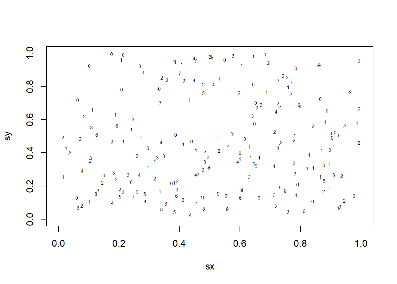

#assume there is no spatial dependenc we might fit a simple non-spatial GLM using
pois.nonsp <- glm(y~1, family = "poisson")
beta.init <- coefficients(pois.nonsp)

##
data <- as.geodata(cbind(s, y), coords.col = 1:2, data.col =3)
mcmc <- mcmc.control(S.scale = 0.55,thin = 20, n.iter=50000, burn.in=1000)
model <- list(cov.pars=c(0.2, -0.5/log(0.05)), beta=beta.init, family="poisson")
outmcmc <- glsm.mcmc(data, model= model, mcmc.input = mcmc,messages = FALSE)
mcmcobj <- prepare.likfit.glsm(outmcmc)
lik <- likfit.glsm(mcmcobj, ini.phi =0.5/-log(0.05), fix.nugget.rel = TRUE, messages = FALSE)
print(lik)

## likfit.glsm: estimated model parameters:
##     beta  sigmasq      phi 
## "0.8144" "0.2728" "0.1823" 
## 
##  likfit.glsm : maximised log-likelihood = 1.058

summary(lik)

## Summary of the maximum likelihood parameter estimation
## -----------------------------------
## Family =  poisson , Link =  log 
## 
## Parameters of the mean component (trend):
##     beta 
## "0.8144" 
## 
## Parameters of the spatial component:
##    correlation function: exponential
## 
##       (estimated) variance parameter sigmasq (partial sill) =  0.2728
##       (estimated) cor. fct. parameter phi (range parameter)  =  0.1823
## 
##  (fixed) relative nugget = 0
## 
## 
## 
## Maximised Likelihood:
##    log.L n.params 
##  "1.058"      "3" 
## 
## Call:
## likfit.glsm(mcmc.obj = mcmcobj, ini.phi = 0.5/-log(0.05), fix.nugget.rel = TRUE, 
##     messages = FALSE)

Remark: It is more popular to do inference and prediction for SGLMM under Bayesian framework. In this section, we mainly focus on understanding the modeling idea of SGLMM. We’ll illustrate more on estimation and predictions in the next section “Hierarchical Bayesian spatial models”.

3.5 Hierarchical Bayesian spatial models

All of the above models, estimations, predictions and inferences are derived from the frequentist statistics, where the model parameters are unknown deterministic constants. In Bayesian statistics, model parameters are considered as random variables sampled from a prior distribution.

Bayesian paradigm has its attractive advantages. It can formally incorporate prior opinion or external empirical evidence; it offers flexibility to model multiple levels of randomness and to incorporate information from different sources, which is useful to model complicated data structures.

3.5.1 Basics of Bayesian inference

Let \(p(\cdot|\cdot)\) denotes a conditional probability density. In Bayesian framework, in addition to specifying the distribution \(p({\mathbf{y}}\, | \, {\boldsymbol{\theta}})\) for the observed data \({\mathbf{y}}= (y_1,..,y_n)^\top\) given the unknown parameters \({\boldsymbol{\theta}}= (\theta_1,...,\theta_q)^\top\), we model \({\boldsymbol{\theta}}\) as random variables with distribution \(p({\boldsymbol{\theta}})\). \(p({\boldsymbol{\theta}})\) is called the prior of \({\boldsymbol{\theta}}\), which usually is related to external knowledge or expert opinion. The prior \(p({\boldsymbol{\theta}})\) often contains a vector of hyperparameters \({\boldsymbol{\lambda}}\). Given \({\boldsymbol{\lambda}}\) known, inference on \({\boldsymbol{\theta}}\) is based on its posterior distribution obtained by Bayes’ rule, \[p({\boldsymbol{\theta}}\, | \, {\mathbf{y}}) = \frac{p({\mathbf{y}},{\boldsymbol{\theta}})}{p({\mathbf{y}})} = \frac{p({\mathbf{y}}\, | \,{\boldsymbol{\theta}})p({\boldsymbol{\theta}})}{\int p({\mathbf{y}}\, | \,{\boldsymbol{\theta}})p({\boldsymbol{\theta}}) d{\boldsymbol{\theta}}}.\] Further, we can see that the denominator is independent of \({\boldsymbol{\theta}}\) and hence the posterior density \(p({\boldsymbol{\theta}}\, | \, {\mathbf{y}})\) is proportional to \(p({\mathbf{y}}\, | \,{\boldsymbol{\theta}})p({\boldsymbol{\theta}})\), i.e., \[p({\boldsymbol{\theta}}\, | \, {\mathbf{y}}) \propto p({\mathbf{y}}\, | \,{\boldsymbol{\theta}})p({\boldsymbol{\theta}}).\]

Here is an example from Gelman et al. (2014).

Example 3.9 (Spelling correction) Suppose that someone types “radom”. How should that be read? It could be a misspelling or mistyping of “random” or “radon” or some other alternative, or it could be the intentional typing of “radom”. What is the probability that “radom” actually means “random”?

If we label \(y\) as the data and \(\theta\) as the word that the person was intending to type. For simplicity, we consider only three possibilities for the intended word \(\theta\) (random, radon, or radom). Then, the posterior density of \(\theta\) is \[p(\theta \, | \, y = ``radom") \propto p(\theta) p(y = ``radom" \, | \, \theta).\]

What would be the prior distribution? Without any other context, it makes sense to assign the prior probabilities based on the relative frequencies of these three words in some large database. Here consider a prior provided by researchers at Google: \[p(\theta = ``random") = 7.6\times 10^{-5},\\ p(\theta = ``radon") = 6.05 \times 10^{-6},\\ p(\theta =``radom") = 3.12\times 10^{-7}.\]

What would be the likelihood \(p(y = ``radom" \, | \, \theta)\)? Here are conditional probabilities from Google’s model of spelling and typing errors: \[p(y = ``radom" \, | \, \theta = ``random") = 0.00193,\\ p(y = ``radom" \, | \, \theta = ``radon") = 0.000143 ,\\ p(y = ``radom" \, | \, \theta = ``radom") = 0.975.\]

Now we can derive the posterior distribution from Bayes’ rule, \[p(\theta = ``random" \, | \, y = ``radom" ) = 0.325,\\ p(\theta = ``radon" \, | \, y = ``radom" ) = 0.002 ,\\ p(\theta = ``radom" \, | \, y = ``radom") = 0.673.\]

As is well known, frequentist statisticians try to construct an estimator of parameter \({\boldsymbol{\theta}}\), say \(\hat {\boldsymbol{\theta}}\), study the (asymptotic) distribution of \(\hat {\boldsymbol{\theta}}\), and then do hypothesis testing and confidence intervals for \({\boldsymbol{\theta}}\). However, in Bayesian statistics, a point estimate of \({\boldsymbol{\theta}}\) can be the mean or median of posterior distribution. Similarly, an interval estimate of \({\boldsymbol{\theta}}\) can be a central interval of posterior density which corresponds to a probability of \(100(1-\alpha)\%\). Such interval estimate is called \(100(1-\alpha)\%\) posterior interval. Hence, once we obtained the posterior distribution of \({\boldsymbol{\theta}}\), Bayesian estimation and inference are straightforward. If we have closed form of \(p({\boldsymbol{\theta}}\, | \, {\mathbf{y}}, {\boldsymbol{\lambda}})\), summaries such as mean, median, standard deviation and posterior interval can be available in closed form. But most of time, when models are complicated, they are computed using computer simulations from the posterior distribution (Monte Carlo Markov Chain (MCMC) methods).

After observing the data \({\mathbf{y}}=(y_1,..,y_n)^\top\), we want to predict the unknown variable, say \(\tilde {\mathbf{y}}\), from the same model. How do we do prediction in Bayesian statistics? Again we will not doing this by finding a predicted value and then learn the distribution of it as done in frequentist statistics. Instead, we derive the posterior predictive distribution, specifically, \[p(\tilde {\mathbf{y}}\, | \, {\mathbf{y}}) = \int p(\tilde {\mathbf{y}}, {\boldsymbol{\theta}}\, | \, {\mathbf{y}})d{\boldsymbol{\theta}}=\int p(\tilde {\mathbf{y}}\, | \, {\boldsymbol{\theta}},{\mathbf{y}})p({\boldsymbol{\theta}}| {\mathbf{y}}) d{\boldsymbol{\theta}}= \int p(\tilde {\mathbf{y}}\, | \, {\boldsymbol{\theta}})p({\boldsymbol{\theta}}\, | \, {\mathbf{y}}) d{\boldsymbol{\theta}}.\] Again, the point predicted value can be the mean or median of the posterior predictive distribution. The \(100(1-\alpha)\%\) prediction interval can be a central interval of posterior predictive density which corresponds to a probability of \(100(1-\alpha)\%\).

Example 3.10 Assume that the data points \({\mathbf{y}}=(y_1,...,y_n)^\top\) follows independent Gaussian distributions with unknown mean \(\mu\) and known variance \(\sigma^2\). The prior density of \(\mu\) is assumed to be Gaussian distribution with mean \(\mu_0\) and variance \(\tau_0^2\), with known hyperparameters \(\mu_0\) and \(\tau_0^2\). Then what is the posterior density of \(\mu\)?

\[p(\mu \, | \, {\mathbf{y}}) \propto p(\mu)p({\mathbf{y}}\, | \,\mu) = p(\mu)\prod_{i=1}^n p(y_i \, | \, \mu)\\ \propto e^{-\frac{(\mu-\mu_0)^2}{2\tau_0^2}}\prod_{i=1}^n e^{-\frac{(y_i-\mu)^2}{2\sigma^2}} \propto e^{-\frac{(\mu-\mu_n)^2}{2\tau_n^2}},\] where \[\mu_n = \frac{\frac{1}{\tau_0^2}\mu_0 + \frac{n}{\sigma^2} \bar y}{\frac{1}{\tau_0^2}+\frac{n}{\sigma^2}}, \ \ \text{and} \ \ \tau_n^2 = \left(\frac{1}{\tau_0^2}+\frac{n}{\sigma^2}\right)^{-1}.\] So the posterior distribution of \(\mu\) given \({\mathbf{y}}\) is Gaussian distribution with mean \(\mu_n\) and variance \(\tau_n^2\).

3.5.2 Hierarchical Bayesian spatial models for Gaussian geostatistical data

Consider the geostatistical data \(y({\mathbf{s}}_1),..., y({\mathbf{s}}_n)\) with exploratory variables (predictors) \({\mathbf{X}}({\mathbf{s}}_i) = (X_1({\mathbf{s}}_i),X_2({\mathbf{s}}_i),...,X_p({\mathbf{s}}_i))^\top, i=1,2,...,n\). Recall the spatial regression model: at any location \({\mathbf{s}}\in \mathcal{D}\), the response variable \(Y\) is modeled by \[Y({\mathbf{s}}) = \beta_0 + X_1({\mathbf{s}})\beta_1 + ... + X_p({\mathbf{s}})\beta_p + w({\mathbf{s}}) + e({\mathbf{s}}) = {\mathbf{X}}({\mathbf{s}})^\top {\boldsymbol{\beta}}+ w({\mathbf{s}})+e({\mathbf{s}}),\] where \({\boldsymbol{\beta}}= (\beta_0,...,\beta_p)^\top\) are unknown coefficients, \(w({\mathbf{s}})\) is a weakly stationary random field with mean zero and covariance function \(C_w({\mathbf{h}}; {\boldsymbol{\theta}})\) and \(e({\mathbf{s}})\) is a white noise with variance \(\sigma_e^2\).

To incorporate the distribution model for parameters \({\boldsymbol{\beta}},{\boldsymbol{\theta}},\sigma_e^2\), we use the Bayesian hierarchical modeling framework,which specify a data model, process model, and parameter models. Specifically,

\[ \begin{align*} \text{data model: } &Y({\mathbf{s}})\, |\, {\boldsymbol{\beta}}, w({\mathbf{s}}), \sigma_e^2 \stackrel{ind.}{\sim} Gaussian({\mathbf{X}}({\mathbf{s}})^\top {\boldsymbol{\beta}}+ w({\mathbf{s}}), \sigma_e^2)\\ \text{process model: }& w({\mathbf{s}})\, |\, {\boldsymbol{\theta}}\sim Gaussian(0, C({\mathbf{h}};{\boldsymbol{\theta}}))\\ \text{parameter model: } & p({\boldsymbol{\beta}}, \sigma_e^2, {\boldsymbol{\theta}}), \end{align*} \] where \(p({\boldsymbol{\beta}}, \sigma_e^2, {\boldsymbol{\theta}})\) is the prior density of \(({\boldsymbol{\beta}},\sigma_e^2,{\boldsymbol{\theta}})^\top\).

More often, people represent the above model in terms of the observed data.Let \(I\) be the identity matrix, \({\mathbf{Y}}=(y(s_1), ..., y({\mathbf{s}}_n))^\top\), \({\mathbf{w}}= (w({\mathbf{s}}_1), ..., w({\mathbf{s}}_n))^\top\), \({\text{Var}}({\mathbf{w}}) = \Sigma({\boldsymbol{\theta}})\),
\[{\mathbf{X}}= \begin{pmatrix} 1 & X_1({\mathbf{s}}_1) &\cdots &X_p({\mathbf{s}}_1)\\ 1& X_1({\mathbf{s}}_2) & \cdots &X_p({\mathbf{s}}_2)\\ \vdots & \vdots & \ddots &\vdots\\ 1& X_1({\mathbf{s}}_n) &\cdots & X_p({\mathbf{s}}_n)\\ \end{pmatrix}.\] Then there is an alternative representation of Bayesian hierarchical model.

\[ \begin{align*} \text{data model: } &{\mathbf{Y}}\, |\, {\boldsymbol{\beta}}, {\mathbf{w}}, \sigma_e^2 \sim Gaussian({\mathbf{X}}{\boldsymbol{\beta}}+ {\mathbf{w}}, \sigma_e^2\mathbf{I})\\ \text{process model: }& {\mathbf{w}}\, |\, {\boldsymbol{\theta}}\sim Gaussian(0,\Sigma({\boldsymbol{\theta}}))\\ \text{parameter model: } & p({\boldsymbol{\beta}}, \sigma_e^2, {\boldsymbol{\theta}}). \end{align*} \]

1. Prior specification.

Typically independent priors are chosen for the different parameters, that is \[p({\boldsymbol{\beta}}, \sigma_e^2, {\boldsymbol{\theta}}) = p({\boldsymbol{\beta}})p(\sigma_e^2)p({\boldsymbol{\theta}}).\]

For the regression coefficients \({\boldsymbol{\beta}}\), the natural candidate prior is multivariate Gaussian with hyperparameters \(\mu_{\boldsymbol{\beta}}\) and \(\Sigma_{\boldsymbol{\beta}}\). Without any additional context, the mean of the multivariate Gaussian is set to zero and the variance matrix is \(\sigma_{\boldsymbol{\beta}}^2 \mathbf{I}\) with very large \(\sigma_{\boldsymbol{\beta}}^2\).

For the variance of nugget effect \(\sigma_e^2\), the natural candidate prior is inverse Gamma with hyperparameters \(a_{\sigma_e^2}\) and \(b_{\sigma_e^2}\). Usually, \(a_{\sigma_e^2} = 2\) and \(b\) is set to be the estimated variance of nugget effect obtained by variogram methods. The density of inverse Gamma is \[p(x;a,b) = \frac{b^a}{\Gamma(a)}x^{-a-1}e^{-b/x}.\] If we choose exponential covariance function, \(C({\mathbf{h}};{\boldsymbol{\theta}}) = \sigma_w^2 e^{-\phi ||h||}\), then the prior of \({\boldsymbol{\theta}}\) will be \[p({\boldsymbol{\theta}}) = p(\sigma_w^2)p(\phi),\] where \(p(\sigma_w^2)\) is usually inverse Gamma with hyperparameter \(a=2\) and \(b\) the estimated \(\sigma_w^2\) from variogram methods, and \(p(\phi)\) is a uniform distribution with lower limit \(-\log(0.05)/d_{max}\) and upper limit \(-\log(0.01)/d_{min}\) where \(d_{max}\) and \(d_{min}\) are maximum and minimum distance across all pairs of locations where \({\mathbf{Y}}\) are observed (see, e.g., Ren and Banerjee (2013)).

Remark: The range of \(\phi\) is \((0,\infty)\). However, the product \(\sigma_w^2 \phi\) can be identified and estimated well but not the individual \(\phi\) or \(\sigma_w^2\). In general, the range parameter \(\phi\) is hard to be estimated accurately. Fortunately, spatial predictions are only sensitive to \(\sigma_w^2 \phi\). To this end, in practice, we usually use a very informative prior for \(\phi\) (uniform distribution with a specified interval) and a relatively vague prior for \(\sigma_w^2\).

2. Bayesian estimation and inference.

The posterior distribution of Bayesian hierarchical model \[p({\boldsymbol{\beta}},{\boldsymbol{\theta}},\sigma_e^2, {\mathbf{w}}\,|\, {\mathbf{Y}}) \propto p({\mathbf{Y}}\,|\, {\boldsymbol{\beta}}, {\mathbf{w}}, \sigma_e^2)p({\mathbf{w}}\,|\,{\boldsymbol{\theta}})p({\boldsymbol{\beta}})p(\sigma_e^2)p({\boldsymbol{\theta}}).\] The above posterior distribution contains the latent variable \({\mathbf{w}}\) whose dimension is the number locations \(n\). For the above Gaussian model, \({\mathbf{w}}\) can be integrated out to obtain a marginal model only containing the parameters, \[p({\boldsymbol{\beta}}, {\boldsymbol{\theta}}, \sigma_e^2\,|\,{\mathbf{Y}}) \propto p({\mathbf{Y}}\,|\,{\boldsymbol{\beta}},\sigma_e^2,{\boldsymbol{\theta}})p({\boldsymbol{\beta}})p(\sigma_e^2)p({\boldsymbol{\theta}}).\] There are no analytical form for the posterior density and Monte Carlo methods must be used to obtain samples from the posterior distribution. Let \({\boldsymbol{\beta}}^{(1)},...,{\boldsymbol{\beta}}^{(k)}\) and \({\boldsymbol{\theta}}^{(1)},...,{\boldsymbol{\theta}}^{(k)}\) are random samples from the posterior distribution \(p({\boldsymbol{\beta}}, {\boldsymbol{\theta}}, \sigma_e^2\,|\,{\mathbf{Y}})\) via MCMC algorithm.

Then, the Bayesian estimate of \({\boldsymbol{\beta}}\) can be the empirical posterior mean \(\hat {\boldsymbol{\beta}}= \frac{1}{n}\sum_{i=1}^k {\boldsymbol{\beta}}^{(i)}\) or the empirical posterior median, that is the median of the sequence \({\boldsymbol{\beta}}^{(1)},...,{\boldsymbol{\beta}}^{(k)}\). The Bayesian interval estimate for \({\boldsymbol{\beta}}\) can be the the empirical 95% posterior interval, that is between \(2.5\)th percentile and \(97.5\)th percentile of the sequence \({\boldsymbol{\beta}}^{(1)},...,{\boldsymbol{\beta}}^{(k)}\). The estimation and inference of \({\boldsymbol{\theta}}\) can be obtained in the same way by using \({\boldsymbol{\theta}}^{(1)},...,{\boldsymbol{\theta}}^{(k)}\).

3. Bayesian prediction.

Recall that there are two types of spatial krigings. One is predicting the signal process without nugget either at existing locations or new locations, that are \(Z({\mathbf{s}})={\mathbf{X}}({\mathbf{s}})^\top {\boldsymbol{\beta}}+ w({\mathbf{s}})\). The other one is predicting \(y\) at new locations, say \(y({\mathbf{s}}_0)\).

To predict the signal process, we should first recover the latent process \(w({\mathbf{s}})\). Suppose that we want to get \(w\) \(\tilde{\mathbf{s}}_1,...,\tilde{\mathbf{s}}_m\) (observed or new locations). Let \({\mathbf{w}}_0 = (w(\tilde {\mathbf{s}}_1), ..., w(\tilde {\mathbf{s}}_m))^\top\). In the Bayesian setting, the posterior realization of \({\mathbf{w}}_0\) can be sampled from \[p({\mathbf{w}}_0 \,|\, {\mathbf{Y}}) = \int p({\mathbf{w}}_0 \,|\, {\boldsymbol{\theta}})p({\boldsymbol{\theta}}\,|\,{\mathbf{Y}})d{\boldsymbol{\theta}}.\] It can be done using composition sampling using posterior samples \({\boldsymbol{\theta}}^{(1)},...,{\boldsymbol{\theta}}^{(k)}\). Specifically, given \({\boldsymbol{\theta}}^{(i)}, i=1,2,..,k\), \({\mathbf{w}}^{(i)}\) can be drawn from the multivariate Gaussian density \(p({\mathbf{w}}\,|\, {\boldsymbol{\theta}}^{(i)})\). The posterior estimate of \({\mathbf{w}}\) can be consider as the mean or median of \({\mathbf{w}}^{(1)},...,{\mathbf{w}}^{(k)}\). And for any \(j=1,2,...,m\), the signal \(Z(\tilde {\mathbf{s}}_j)\) can be predicted via posterior mean of \({\mathbf{X}}(\tilde {\mathbf{s}}_j)^\top{\boldsymbol{\beta}}^{(1)} + w(\tilde s_j)^{(1)},...,{\mathbf{X}}(\tilde {\mathbf{s}}_j)^\top{\boldsymbol{\beta}}^{(k)} + w(\tilde s_j)^{(k)}\).

To do the prediction of \(y\) at new location \({\mathbf{s}}_0\), we can obtain the samples from the posterior predictive distribution, \[p(y({\mathbf{s}}_0)\,|\, {\mathbf{Y}}, {\mathbf{X}}({\mathbf{s}}_0)) = \int p(y({\mathbf{s}}_0) \,|\, {\mathbf{Y}}, {\boldsymbol{\beta}}, {\boldsymbol{\theta}}, {\mathbf{X}}({\mathbf{s}}_0)) p({\boldsymbol{\beta}}, {\boldsymbol{\theta}}\,|\, {\mathbf{Y}})d{\boldsymbol{\theta}}.\] It can also be obtained via composition sampling using posterior samples \({\boldsymbol{\beta}}^{(1)},{\boldsymbol{\theta}}^{(1)},...,{\boldsymbol{\beta}}^{(k)}, {\boldsymbol{\theta}}^{(k)}\). Specifically, given \({\boldsymbol{\beta}}, {\boldsymbol{\theta}}^{(i)}, i=1,2,..,k\), \(y({\mathbf{s}}_0)^{(i)}\) can be drawn from the multivariate Gaussian density \(p(y({\mathbf{s}}_0) \,|\,{\mathbf{Y}}, {\boldsymbol{\theta}}^{(i)}, {\mathbf{X}}({\mathbf{s}}_0))\). The posterior prediction of \(y({\mathbf{s}}_0)\) can be consider as the mean or median of \(y({\mathbf{s}}_0)^{(1)},...,y({\mathbf{s}}_0)^{(k)}\).

4. Bayesian computation.

The principle of Bayesian estimation, inference and prediction are not hard to understand. However, the main challenge is how to obtain a sample from the posterior distributions which usually do not have close form. The most widely used tools in practice are Markov chain Monte Carlo (MCMC) methods. The MCMC algorithms generates Markov chains of \({\boldsymbol{\theta}}\) and \({\boldsymbol{\beta}}\) whose limiting distributions equal to the posterior distributions of \({\boldsymbol{\theta}}\) and \({\boldsymbol{\beta}}\). So an ideal sample of \({\boldsymbol{\theta}}\) and \({\boldsymbol{\beta}}\) should be subsequences of Markov chains after convergence.

However, this convergence is the most difficult part while implementing MCMC methods. First, we have to decide from which iteration the Markov chain starts to converge to the posterior distribution. Second, the sample drawn from Markov chain are correlated. As a result, standard error estimate would be not accurate with the MCMC posterior sample.

Now we’ll use the following example to explain the details of implementation of Bayesian spatial regression models.

Example 3.11 (Biomass vs. LiDAR) Forestry scientists are interested in mapping the tree biomass, at a high spatial resolution with associated, spatially-explicit uncertainty. The LiDAR signal is a good covariate to improve the prediction of biomass. Strong signals far away from the ground indicate a large amount of biomass (tall trees); Strong signals around the ground indicates a small amount of biomass (small trees) (see the above figure from https://daac.ornl.gov/CMS/guides/CMS_LiDAR_AGB_PEF_2012.html).

The study area is the US Forest Service Penobscot Experimental Forest (PEF; www.fs.fed.us/ne/durham/4155/penobsco.htm), ME, USA. The dataset comprises LiDAR waveforms collected with the Laser Vegetation Imaging Sensor (LVIS; http://lvis.gsfc.nasa.gov) and several forest variables measured on a set of 589 georeferenced forest inventory plots, including biomass. The first four principle compenents of LiDAR signals, which explain over 90% of the signal variance, were substracted from LiDAR data and saved in “LiDAR_pca.csv”. We want to use principle compenents of LiDAR signals to improve the prediction of biomass in high resolution.

The details of this example can be found at http://blue.for.msu.edu/GC14/exercises/exercise-spLM/initial-exploration-spLM.pdf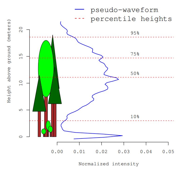

We first do data visualization and exploratory data analysis.

# R codes mainly from 
#http://blue.for.msu.edu/GC14/exercises/exercise-spLM/initial-exploration-spLM.R

rm(list=ls())
library(yaImpute)
library(spBayes)
library(MBA)
library(geoR)
library(fields)
library(rgdal)
library(RgoogleMaps)
library(raster)

#get data
PEF.shp <- readOGR("./data/PEF-data","PEF-bounds")

## OGR data source with driver: ESRI Shapefile 
## Source: "C:\Users\yzhou\Box Sync\STAT-432-831-Spring-2020\lecture notes\github\Spatial_Statistics_Lecture_Notes\data\PEF-data", layer: "PEF-bounds"
## with 1 features
## It has 5 fields
## Integer64 fields read as strings:  ID ACRES

proj4string(PEF.shp) <- CRS("+proj=utm +zone=18 +ellps=WGS84
                            +datum=WGS84 +units=m +no_defs") ## set the projection
PEF.poly <- as.matrix(PEF.shp@polygons[[1]]@Polygons[[1]]@coords)

PEF.plots <- read.csv("./data/PEF-data/PEF-plots.csv")

##drop rows with NA biomass
PEF.plots <- PEF.plots[sapply(PEF.plots[,"biomass.mg.ha"],
                              function(x){!any(is.na(x))}),]

##get plot coordinates and transform biomass
coords <- PEF.plots[,c("easting", "northing")]
bio <- sqrt(PEF.plots$biomass.mg.ha)

##plot
plot(coords, pch=19, cex=0.5, xlab="Easting (m)", ylab="Northing (m)")
plot(PEF.shp, add=TRUE)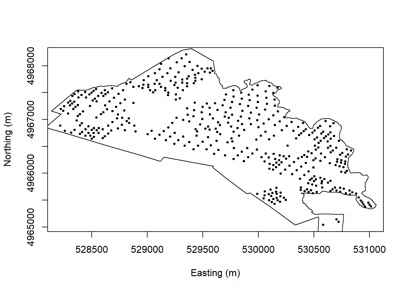

b.box <- as.vector(t(bbox(PEF.shp)))
surf <- mba.surf(cbind(coords, bio), no.X=200, no.Y=200,
                 extend=TRUE, b.box=b.box, sp=TRUE)$xyz.est
proj4string(surf) <- CRS("+proj=utm +zone=18 +ellps=WGS84
                         +datum=WGS84 +units=m +no_defs")
surf <- as.image.SpatialGridDataFrame(surf[PEF.shp,])
image.plot(surf, xaxs = "r", yaxs = "r", xlab="Easting (m)", ylab="Northing (m)")
plot(PEF.shp, add=TRUE)
points(coords)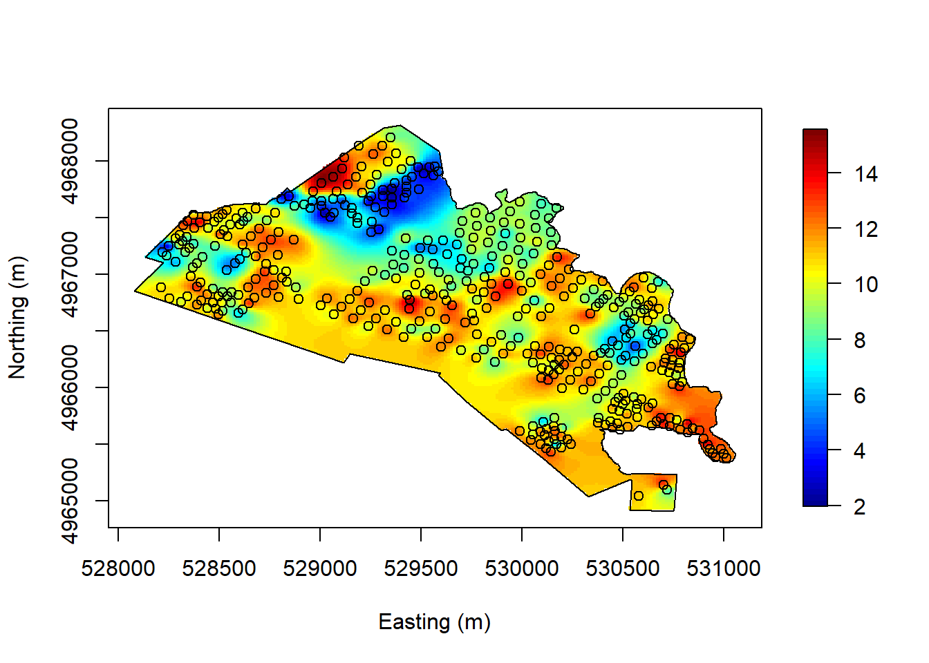

#read in LiDAR coords and PCs.
lidar <- read.csv("./data/LiDAR_pca.csv", header = TRUE)
lidar.coords <- lidar[,1:2]
Z <- lidar[,3:6]

##match lidar coords to biomass coords
X <- as.matrix(Z[ann(as.matrix(lidar.coords),
                     as.matrix(coords))$knnIndexDist[,1],])

## Target points completed: 
##      100...200...300...400...

##try non-spatial model and get the residual plot.
bio <- sqrt(PEF.plots$biomass.mg.ha)

m <- lm(bio ~ X)
summary(m)

## 
## Call:
## lm(formula = bio ~ X)
## 
## Residuals:
##     Min      1Q  Median      3Q     Max 
## -5.7752 -0.9775  0.1600  1.2460  5.6735 
## 
## Coefficients:
##               Estimate Std. Error t value Pr(>|t|)    
## (Intercept)   10.05107    0.09411 106.804  < 2e-16 ***
## XPC1        -170.33901   10.45809 -16.288  < 2e-16 ***
## XPC2         -93.70959   11.03247  -8.494 3.01e-16 ***
## XPC3          -0.81924   11.50711  -0.071    0.943    
## XPC4           4.88962    9.93443   0.492    0.623    
## ---
## Signif. codes:  0 '***' 0.001 '**' 0.01 '*' 0.05 '.' 0.1 ' ' 1
## 
## Residual standard error: 1.933 on 446 degrees of freedom
## Multiple R-squared:  0.4019, Adjusted R-squared:  0.3965 
## F-statistic: 74.91 on 4 and 446 DF,  p-value: < 2.2e-16

bio.resid <- resid(m)

resid.surf <- mba.surf(cbind(coords, bio.resid), no.X=200,
                       no.Y=200, extend=TRUE, b.box=b.box, sp=TRUE)$xyz.est
proj4string(resid.surf) <- CRS("+proj=utm +zone=18
                               +ellps=WGS84 +datum=WGS84 +units=m +no_defs")
resid.surf <- as.image.SpatialGridDataFrame(resid.surf[PEF.shp,])
image.plot(resid.surf, xaxs = "r", yaxs = "r",main =
"residuals", xlab="Easting (m)", ylab="Northing (m)")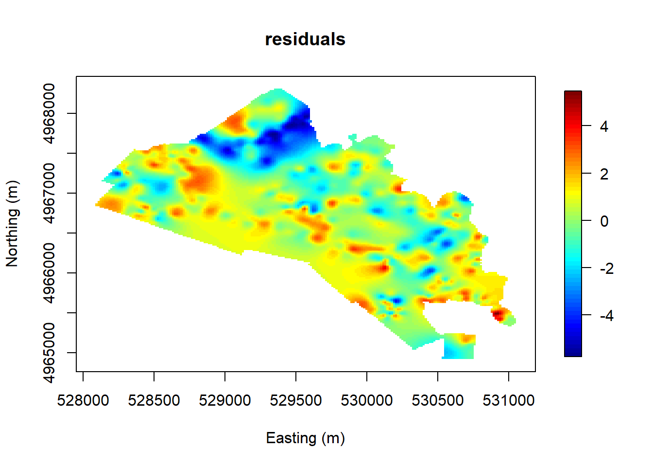

#empirical variograms
#empirical variograms
max.dist <-  0.5 * max(iDist(coords))
m1 <- lm(bio~X)
m1.sum <- summary(m1)
#apply variogram methods
bins <- 100
#Matheron estimator
vario.M <- variog(coords = coords, data = bio, trend = ~X,
                  estimator.type = "classical", uvec = (seq(0, max.dist, l = bins )))

## variog: computing omnidirectional variogram

#Cressie-Hawkins estimator
vario.CH <- variog(coords = coords, data = bio, trend = ~X,
                   estimator.type = "modulus", uvec = (seq(0, max.dist, l = bins )))

## variog: computing omnidirectional variogram

plot(vario.M, main = "bio")
points(vario.CH$u, vario.CH$v, col = "red")
legend("bottomright", legend=c("Matheron", "Cressie-Hawkins"), pch = c(1,1),
       col = c("black", "red"), cex = 0.6)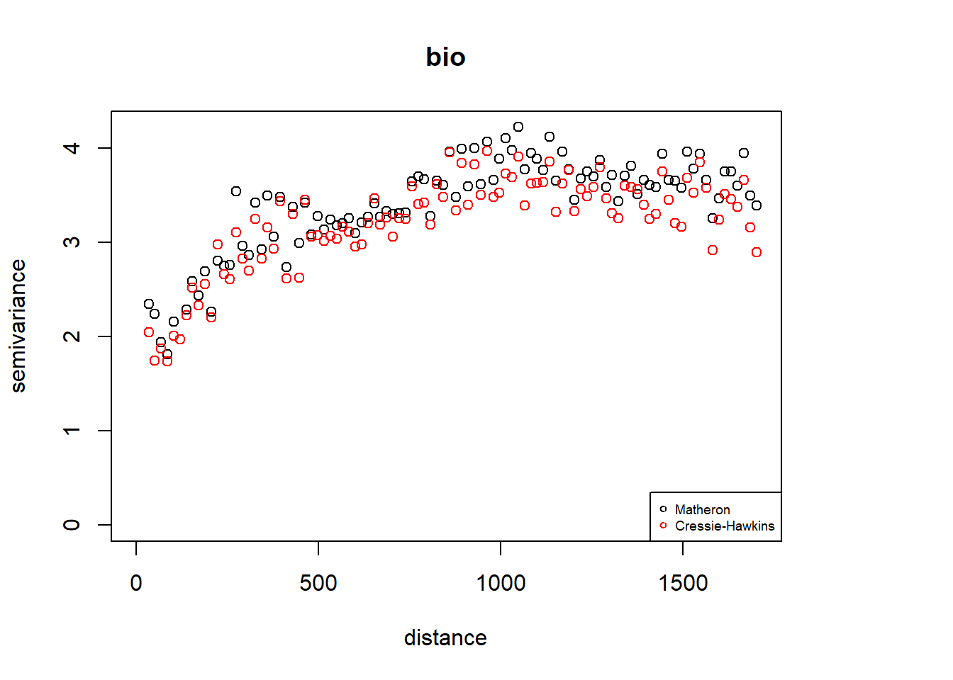

#WLS with weights N(h)/gamma^2(h)
fit.vario <- variofit(vario.M, ini.cov.pars = c(m1.sum$sigma^2,
-max.dist/log(0.05)), cov.model = "exponential", minimisation.function
= "optim", weights = "cressie", control = list(factr=1e-10, maxit = 500),
messages = FALSE)

fit.vario

## variofit: model parameters estimated by WLS (weighted least squares):
## covariance model is: exponential
## parameter estimates:
##    tausq  sigmasq      phi 
##   1.6815   2.1192 340.3413 
## Practical Range with cor=0.05 for asymptotic range: 1019.571
## 
## variofit: minimised weighted sum of squares = 342.4271

#blue line: nugget; green line: sill; red line: effective range
plot(vario.M, main="biomass")
lines(fit.vario)
abline(h=fit.vario$nugget, col="blue")##nugget
abline(h=fit.vario$cov.pars[1]+fit.vario$nugget, col="green")##sill
abline(v=-log(0.05)*fit.vario$cov.pars[2], col="red3")##effective range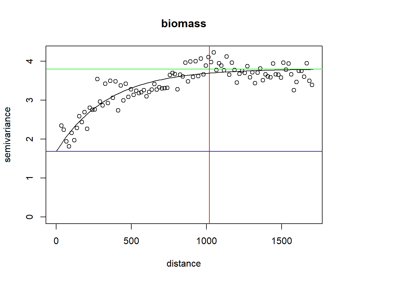

Now use function “spLM” in the package “spBayes” to fit the data with Bayesian spatial regression model. The “spLM” function returns the posterior estimate of covariance parameters \({\boldsymbol{\theta}}\). Here we use exponential covariance function, i.e., \(C({\mathbf{h}};{\boldsymbol{\theta}}) = \sigma_w^2 e^{-\phi ||h||}\).

#Bayesian spatial regression models
#training and testing sets
set.seed(1)
ns <- nrow(coords)
sIndx <- sample(1:ns, 0.75*ns)
s.train <- coords[sIndx, ]
s.test <- coords[-sIndx, ]
bio.train <- bio[sIndx]
bio.test <- bio[-sIndx]
X.train <- X[sIndx, ]
X.test <- X[-sIndx, ]
plot(s.train)
points(s.test, col ="red")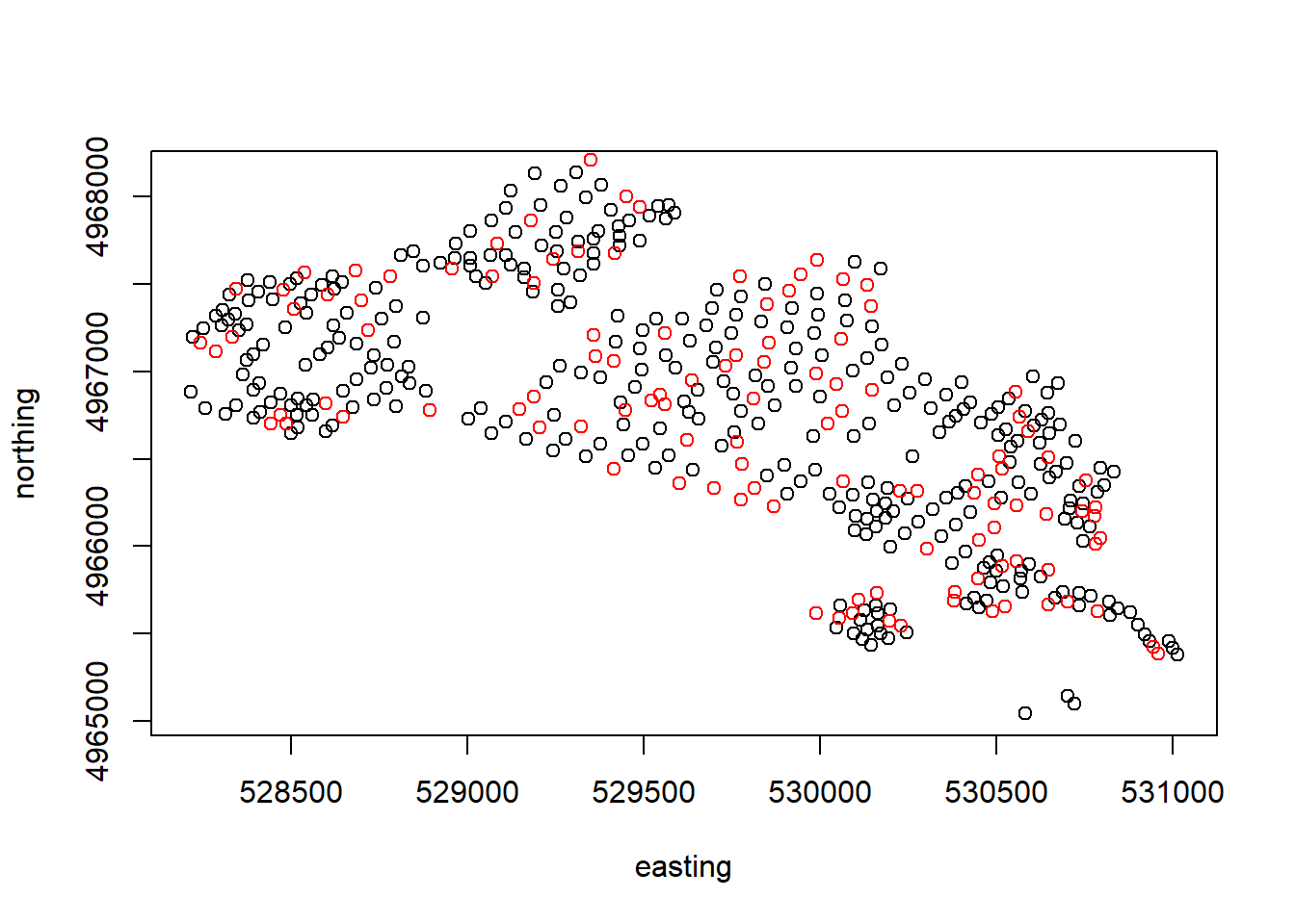

#use exponential covariance. In spBayes package, exponential covariance
#is defined as C(h) = \sigma^2 e^{-\phi |h|}.
n.samples <- 20000
#pick the variogram estimate as the starting value.
starting <- list("phi"=1/fit.vario$cov.pars[2], "sigma.sq"=
                   fit.vario$cov.pars[1], "tau.sq"=fit.vario$nugget)

tuning <- list("phi"=0.5, "sigma.sq"=0.01, "tau.sq"=0.01)

p <- ncol(X.train)+1

dis <- iDist(s.train)
max.dist <- max(dis)
min.dist <- min(dis[dis!=0])
priors <- list("beta.Norm"=list(rep(0,p), diag(1000000,p)),
               "phi.Unif"=c(-log(0.05)/max.dist, -log(0.01)/min.dist), 
"sigma.sq.IG"=c(2, fit.vario$cov.pars[1]),  "tau.sq.IG"=c(2, fit.vario$nugget))

ptm <- proc.time()
m.1 <- spLM(bio.train ~ X.train, coords=as.matrix(s.train), starting=starting,
            tuning=tuning, priors=priors, cov.model="exponential",
            n.samples=n.samples, n.report=floor(n.samples/4))

## ----------------------------------------
##  General model description
## ----------------------------------------
## Model fit with 338 observations.
## 
## Number of covariates 5 (including intercept if specified).
## 
## Using the exponential spatial correlation model.
## 
## Number of MCMC samples 20000.
## 
## Priors and hyperpriors:
##  beta normal:
##  mu: 0.000   0.000   0.000   0.000   0.000   
##  cov:
##  1000000.000 0.000   0.000   0.000   0.000   
##  0.000   1000000.000 0.000   0.000   0.000   
##  0.000   0.000   1000000.000 0.000   0.000   
##  0.000   0.000   0.000   1000000.000 0.000   
##  0.000   0.000   0.000   0.000   1000000.000 
## 
##  sigma.sq IG hyperpriors shape=2.00000 and scale=2.11917
##  tau.sq IG hyperpriors shape=2.00000 and scale=1.68148
##  phi Unif hyperpriors a=0.00088 and b=0.15342
## -------------------------------------------------
##      Sampling
## -------------------------------------------------
## Sampled: 5000 of 20000, 25.00%
## Report interval Metrop. Acceptance rate: 28.76%
## Overall Metrop. Acceptance rate: 28.76%
## -------------------------------------------------
## Sampled: 10000 of 20000, 50.00%
## Report interval Metrop. Acceptance rate: 29.66%
## Overall Metrop. Acceptance rate: 29.21%
## -------------------------------------------------
## Sampled: 15000 of 20000, 75.00%
## Report interval Metrop. Acceptance rate: 29.02%
## Overall Metrop. Acceptance rate: 29.15%
## -------------------------------------------------
## Sampled: 20000 of 20000, 100.00%
## Report interval Metrop. Acceptance rate: 29.32%
## Overall Metrop. Acceptance rate: 29.19%
## -------------------------------------------------

proc.time() - ptm

##    user  system elapsed 
##  152.12    0.19  157.65

The “spLM” function above applied Gibbs sampling and Metropolis-Hasting algorithm to generate the posterior samples. The acceptance rate of Metropolis algorithm cannot be too high or too low, either of which leads to slow convergence of Markov Chains. Usually it could be between 20%-50%. The acceptance rate can be adjusted by changing the tuning parameters. If sometimes it is not easy to tune the chains, we can use adaptive MCMC methods to let the algorithm adjusting the tuning parameters during the sampling process. To this end, we can add the “amcmc” option in “spLM” function.

#amcmc
n.batch <- 400
batch.length <- 50
n.samples <- n.batch*batch.length

m.2 <- spLM(bio.train ~ X.train, coords=as.matrix(s.train), starting=starting,
            tuning=tuning, priors=priors, cov.model="exponential",
            amcmc=list("n.batch"=n.batch, "batch.length"=batch.length, "accept.rate"=0.43),
            n.report=floor(n.batch/4))

## ----------------------------------------
##  General model description
## ----------------------------------------
## Model fit with 338 observations.
## 
## Number of covariates 5 (including intercept if specified).
## 
## Using the exponential spatial correlation model.
## 
## Using adaptive MCMC.
## 
##  Number of batches 400.
##  Batch length 50.
##  Target acceptance rate 0.43000.
## 
## Priors and hyperpriors:
##  beta normal:
##  mu: 0.000   0.000   0.000   0.000   0.000   
##  cov:
##  1000000.000 0.000   0.000   0.000   0.000   
##  0.000   1000000.000 0.000   0.000   0.000   
##  0.000   0.000   1000000.000 0.000   0.000   
##  0.000   0.000   0.000   1000000.000 0.000   
##  0.000   0.000   0.000   0.000   1000000.000 
## 
##  sigma.sq IG hyperpriors shape=2.00000 and scale=2.11917
##  tau.sq IG hyperpriors shape=2.00000 and scale=1.68148
##  phi Unif hyperpriors a=0.00088 and b=0.15342
## -------------------------------------------------
##      Sampling
## -------------------------------------------------
## Batch: 100 of 400, 25.00%
##  parameter   acceptance  tuning
##  sigma.sq    50.0        0.26117
##  tau.sq      62.0        0.26117
##  phi     38.0        0.54522
## -------------------------------------------------
## Batch: 200 of 400, 50.00%
##  parameter   acceptance  tuning
##  sigma.sq    30.0        0.33872
##  tau.sq      32.0        0.39749
##  phi     50.0        0.49333
## -------------------------------------------------
## Batch: 300 of 400, 75.00%
##  parameter   acceptance  tuning
##  sigma.sq    46.0        0.31899
##  tau.sq      40.0        0.39749
##  phi     34.0        0.51346
## -------------------------------------------------
## Batch: 400 of 400, 100.00%
##  parameter   acceptance  tuning
##  sigma.sq    38.0        0.33201
##  tau.sq      40.0        0.38190
##  phi     38.0        0.50330
## -------------------------------------------------

After obtaining the posterior sample of \({\boldsymbol{\theta}}\), we use the function “spRecover” to get the posterior sample of regression coefficients \({\boldsymbol{\beta}}\) and the spatial random field \(w({\mathbf{s}})\). Then, we summarize the Bayesian estimate.

#get beta and spatial random field w
#"Burn-in"" is a term that describes the practice of throwing away some iterations at 
#the beginning of an MCMC run. After the burn-in period, the following MCMC
#sequence would be used as posterior samples. 
burn.in <- 0.75*n.samples
ptm <- proc.time()
m.1 <- spRecover(m.1, start=burn.in, thin=10, verbose=FALSE)
proc.time() - ptm

##    user  system elapsed 
##   41.04    0.04   41.81

m.2 <- spRecover(m.2, start=burn.in, thin=10, verbose=FALSE)
#the option "thin": #a sample thinning factor. The default 
#of 1 considers all samples between start and end. For example, 
#if thin = 10 then 1 in 10 samples are considered between start and end.

#posterior sample of theta
theta.samps <- mcmc.list(m.1$p.theta.samples, m.2$p.theta.samples)
plot(theta.samps, density=FALSE)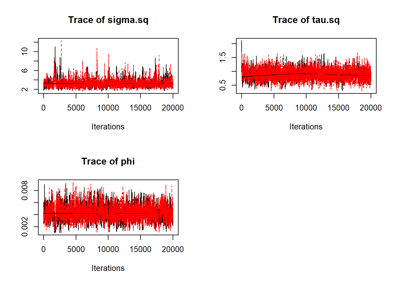

#posterior sample of beta
beta.samps <- mcmc.list(m.1$p.beta.recover.samples, m.2$p.beta.recover.samples)
plot(beta.samps, density=FALSE)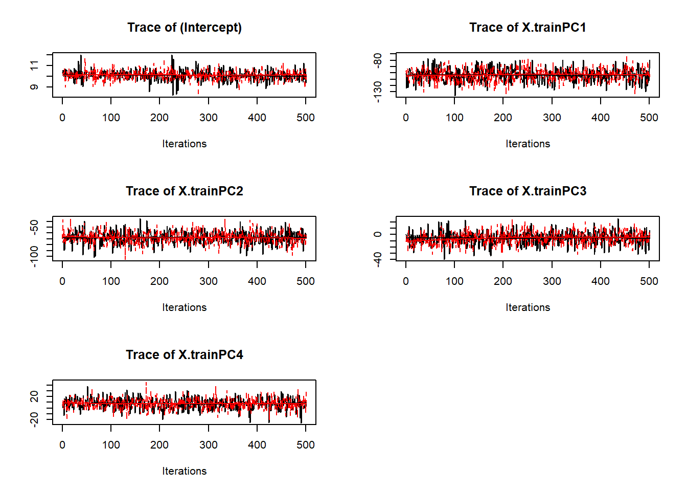

#summary of theta
theta.samps <- mcmc.list(m.1$p.theta.recover.samples, m.2$p.theta.recover.samples)
round(summary(theta.samps)$quantiles,3)

##           2.5%   25%   50%   75% 97.5%
## sigma.sq 2.178 2.782 3.166 3.675 5.579
## tau.sq   0.536 0.747 0.874 0.999 1.262
## phi      0.002 0.003 0.004 0.005 0.007

#recovered w
m.1.w <- m.1$p.w.recover.samples
m.2.w <- m.2$p.w.recover.samples

w.samps <- cbind(m.1.w, m.2.w)

w.summary <- apply(w.samps, 1, function(x){quantile(x, prob=c(0.025,0.5,0.975))})

w.surf <- mba.surf(cbind(s.train, w.summary[2,]), no.X=200, no.Y=200, 
                   extend=TRUE, b.box=b.box, sp=TRUE)$xyz.est
proj4string(w.surf) <- CRS("+proj=utm +zone=18 +ellps=WGS84 +datum=WGS84 +units=m +no_defs")
w.surf <- as.image.SpatialGridDataFrame(w.surf[PEF.shp,])

z.lim <- range(w.surf[["z"]], na.rm=TRUE)

image.plot(w.surf, zlim=z.lim, xaxs = "r", yaxs = "r", main="Spatial random effects", 
           xlab="Easting (m)", ylab="Northing (m)")
plot(PEF.shp, add=TRUE, usePolypath = FALSE)
points(s.train)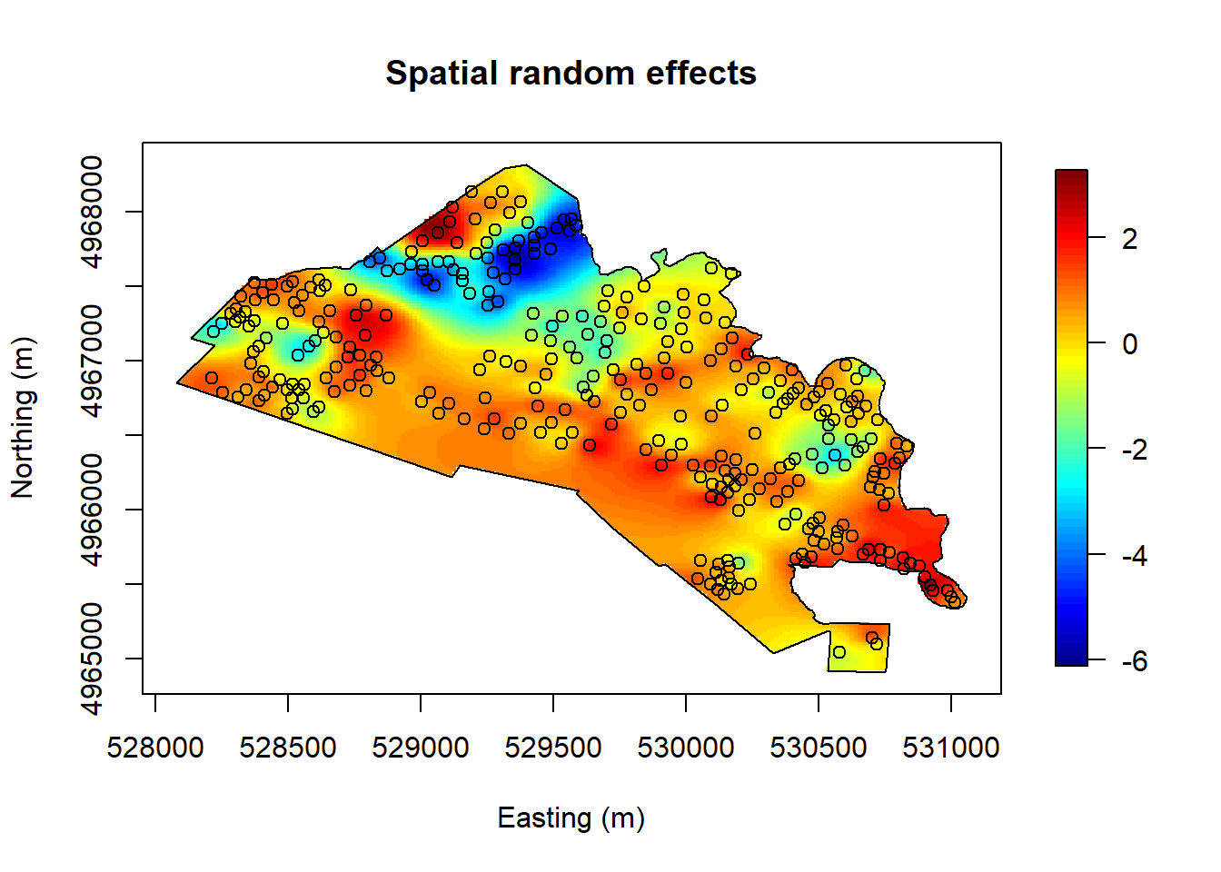

Now we are ready to do Bayesian prediction. We first predict \(\sqrt{biomass}\) at testing locations “s.test”. Then we predict unobserved biomass at high resolutions using the densely sampled LiDAR signals.

#prediction at s.test
pred <- spPredict(m.1, start = burn.in, thin = 10, pred.coords = s.test,
                  pred.covars = cbind(1,X.test))

## ----------------------------------------
##  General model description
## ----------------------------------------
## Model fit with 338 observations.
## 
## Prediction at 113 locations.
## 
## Number of covariates 5 (including intercept if specified).
## 
## Using the exponential spatial correlation model.
## 
## -------------------------------------------------
##      Sampling
## -------------------------------------------------
## Sampled: 100 of 501, 19.76%
## Sampled: 200 of 501, 39.72%
## Sampled: 300 of 501, 59.68%
## Sampled: 400 of 501, 79.64%
## Sampled: 500 of 501, 99.60%

#posterior predicted value and prediction interval
pred.summary <- apply(pred$p.y.predictive.samples, 1,
                      function(x){quantile(x, prob=c(0.025,0.5,0.975))})
pred.summary

##            [,1]      [,2]      [,3]      [,4]      [,5]      [,6]      [,7]
## 2.5%   7.669144  8.961095  7.817364  7.673388  7.018673  7.502338  7.689914
## 50%   10.937176 11.431792 11.038135 10.506189 10.377800 10.225339 10.455789
## 97.5% 14.223595 14.167877 14.745311 13.605919 13.519513 13.464813 13.886571
##           [,8]      [,9]     [,10]     [,11]     [,12]     [,13]     [,14]
## 2.5%   7.96331  9.766369  8.156772  7.750353  6.835399  5.060404  5.439809
## 50%   10.69833 12.657493 10.833628 10.195007  9.216697  7.645859  8.015214
## 97.5% 13.78546 15.403651 13.560382 12.674145 11.932160 10.221937 10.578561
##           [,15]    [,16]    [,17]     [,18]     [,19]     [,20]     [,21]
## 2.5%   5.938683 4.532261 4.740316  5.209877  5.302779  8.550606  9.713886
## 50%    8.405432 7.236274 7.493973  7.722678  8.179126 11.280635 12.517257
## 97.5% 10.931502 9.696993 9.756639 10.142735 11.153103 13.995860 15.344654
##          [,22]     [,23]     [,24]     [,25]     [,26]     [,27]     [,28]
## 2.5%  10.49609  7.754326  7.044652  9.496874  7.311882  7.012656  5.961156
## 50%   13.07941 10.761169 10.106669 12.271743 10.089997  9.626063  8.854876
## 97.5% 15.57594 13.729599 13.319953 14.999739 13.091470 11.961477 11.872333
##           [,29]     [,30]     [,31]     [,32]    [,33]     [,34]     [,35]
## 2.5%   7.637382  9.317475  9.443625  6.893973 10.06483  8.519529  7.372597
## 50%   10.028045 12.115500 11.867124  9.470387 12.79293 11.009960  9.762142
## 97.5% 12.438407 14.799567 14.578475 11.967737 15.48527 13.468476 12.404989
##          [,36]     [,37]     [,38]    [,39]     [,40]     [,41]     [,42]
## 2.5%   8.04734  6.992276  7.363715 10.41916  4.840841  7.480938  5.689332
## 50%   10.25809  9.473273 10.156006 13.11363  7.696164 10.116404  8.321827
## 97.5% 12.62440 11.775292 13.105701 15.70431 10.361158 13.021472 10.625007
##           [,43]     [,44]     [,45]     [,46]     [,47]     [,48]     [,49]
## 2.5%   5.775587  4.477100  6.516084  7.753599  8.412702  7.633963  7.985603
## 50%    8.494749  7.469994  9.322351 10.724632 11.399441 10.541038 10.965014
## 97.5% 11.289124 10.197811 12.508234 13.433050 14.593351 13.071943 13.707347
##           [,50]     [,51]     [,52]     [,53]     [,54]     [,55]     [,56]
## 2.5%   7.357552  6.537570  7.891815  7.324493  6.946624  7.593246  8.877088
## 50%   10.204739  9.108603 10.358588 10.074058  9.670706 10.338013 11.562395
## 97.5% 12.856595 11.757868 12.593307 12.516427 12.446549 12.903552 14.034970
##           [,57]     [,58]     [,59]     [,60]     [,61]     [,62]    [,63]
## 2.5%   7.421935  8.477162  7.816334  7.545409  8.979073  8.656604  8.40520
## 50%   10.184334 11.008573 10.428518 10.025094 11.427167 11.542023 10.88013
## 97.5% 13.075755 13.625576 13.247666 12.367890 14.202114 14.195895 13.23988
##           [,64]     [,65]     [,66]     [,67]    [,68]    [,69]     [,70]
## 2.5%   8.304944  9.608137  7.700821  6.765054  7.94655 10.10375  6.598549
## 50%   11.073311 12.165411 10.337161  9.650888 10.72380 13.05745  9.689333
## 97.5% 13.664305 14.587060 12.599009 12.567573 13.57590 15.82388 13.039146
##           [,71]    [,72]     [,73]     [,74]     [,75]    [,76]     [,77]
## 2.5%   5.736729 10.66177  7.752361  9.110106  9.369056 10.70861  8.005718
## 50%    8.643777 13.13248 10.201292 11.852563 12.022292 13.23200 10.603550
## 97.5% 11.520948 15.79847 12.978232 14.454035 14.565818 15.98674 13.536459
##           [,78]     [,79]     [,80]     [,81]    [,82]     [,83]     [,84]
## 2.5%   9.733526  5.361636  5.155185  5.067930 3.792124  6.353672  5.981181
## 50%   12.671970  8.620344  8.173248  7.405873 6.644539  8.938651  8.655503
## 97.5% 15.093000 11.144608 11.352069 10.665082 9.489150 11.594389 11.524712
##           [,85]     [,86]     [,87]    [,88]    [,89]    [,90]    [,91]
## 2.5%   6.613645  6.654170  5.536039 3.249580 2.069078 3.643897 2.610821
## 50%    9.972159  9.539725  9.417916 5.826463 4.556933 6.251022 5.203719
## 97.5% 12.976507 12.746444 12.572844 8.313574 7.205689 8.839237 7.669697
##           [,92]     [,93]    [,94]     [,95]     [,96]     [,97]     [,98]
## 2.5%  0.6748465 0.7947022 2.275360  5.211943  5.196204  8.828798  5.558601
## 50%   3.3677729 3.7329462 4.905899  7.935799  8.064589 11.526937  8.533192
## 97.5% 5.9299002 6.3305403 7.306544 10.834195 11.060819 14.242754 11.284437
##           [,99]    [,100]    [,101]    [,102]    [,103]    [,104]    [,105]
## 2.5%   5.753617  7.121617  6.018986  6.264442  9.154704  7.963168  7.913751
## 50%    8.725950  9.774060  9.240511  9.034586 12.307414 10.985265 10.905196
## 97.5% 11.561599 13.094510 12.036157 11.924968 15.553142 13.670567 13.989904
##         [,106]    [,107]   [,108]    [,109]    [,110]    [,111]    [,112]
## 2.5%   8.49297  5.998000  7.66456  8.178645  9.115305  5.169751  6.663580
## 50%   11.20876  8.649281 10.53376 11.137749 11.783913  7.876962  9.411255
## 97.5% 14.01028 11.341028 13.22911 14.056745 14.679594 10.795063 12.129337
##          [,113]
## 2.5%   8.585286
## 50%   11.065660
## 97.5% 13.812124

#compare bio.test and predicted median of bio.test
plot(bio.test, pred.summary[2,])
abline(a = 0, b = 1)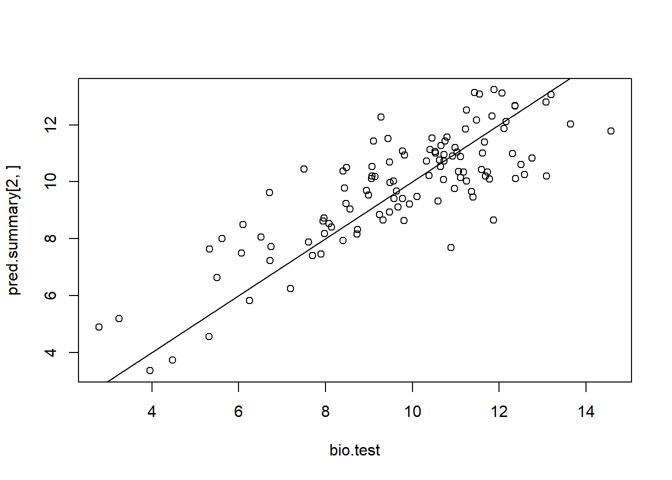

##resample to a regular grid and predict biomass at high resolution
#bounds of lidar coords
bounds <-  as.vector(t(bbox(PEF.shp)))
pix.dim <- 20

pred.coords <- as.matrix(expand.grid(seq(bounds[1], bounds[2], pix.dim), 
                                     seq(bounds[3], bounds[4], pix.dim)))

##subset using the PEF boundary
pred.coords <- pred.coords[pointsInPoly(PEF.poly, pred.coords),]
plot(pred.coords, cex = 0.0001)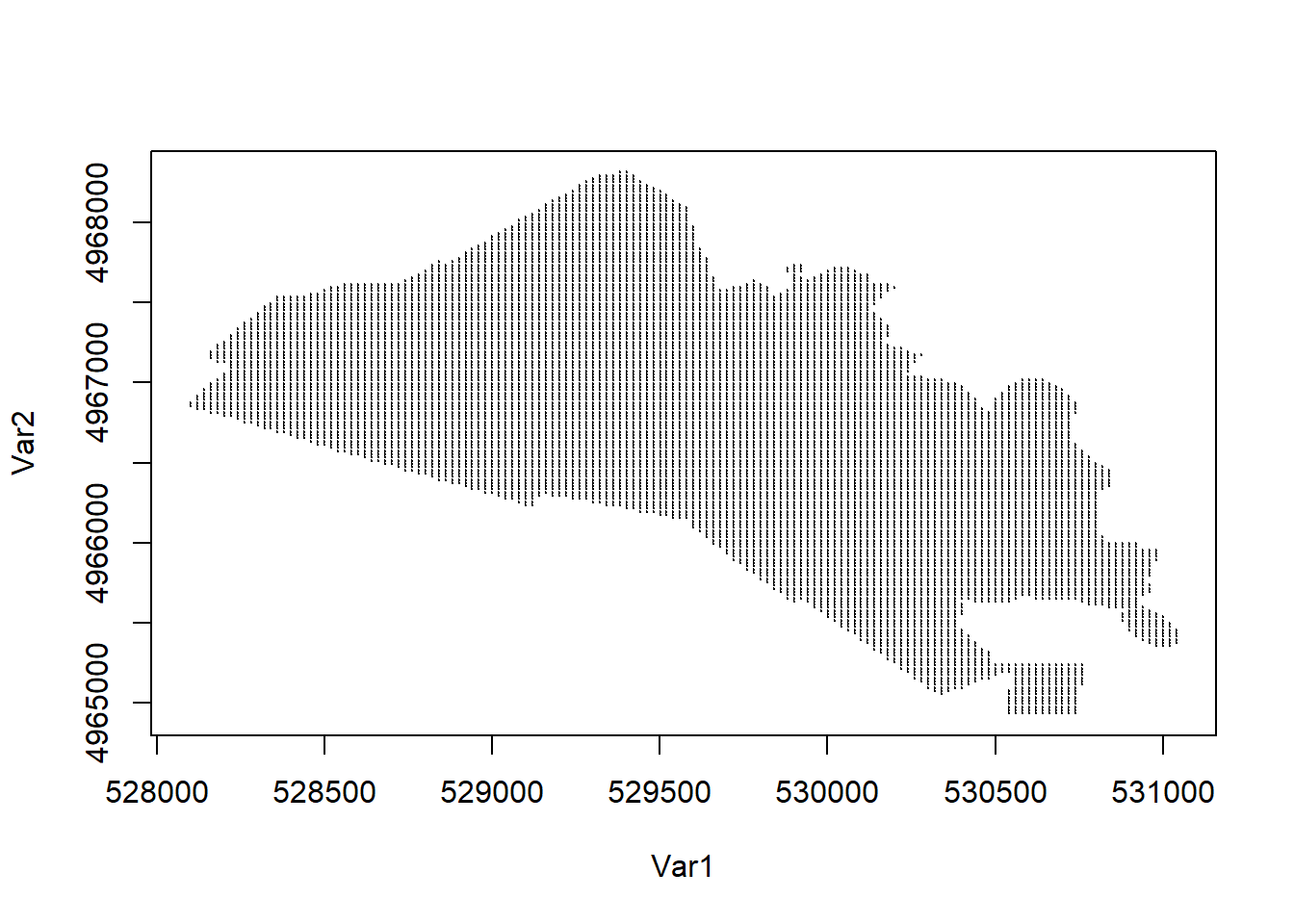

#get the LiDAR PCs at prediction locations.
pred.X <- as.matrix(Z[ann(as.matrix(lidar.coords), as.matrix(pred.coords), 
                          verbose=FALSE)$knnIndexDist[,1],])

pred <- spPredict(m.1, start=burn.in, thin=10, pred.coords=pred.coords, 
                  pred.covars=cbind(1,pred.X))

## ----------------------------------------
##  General model description
## ----------------------------------------
## Model fit with 338 observations.
## 
## Prediction at 10859 locations.
## 
## Number of covariates 5 (including intercept if specified).
## 
## Using the exponential spatial correlation model.
## 
## -------------------------------------------------
##      Sampling
## -------------------------------------------------
## Sampled: 100 of 501, 19.76%
## Sampled: 200 of 501, 39.72%
## Sampled: 300 of 501, 59.68%
## Sampled: 400 of 501, 79.64%
## Sampled: 500 of 501, 99.60%

#posterior prediction median and 95% posterior prediction interval
pred.summary <- apply(pred$p.y.predictive.samples, 1, 
                      function(x){quantile(x, prob=c(0.025,0.5,0.975))})

#visiualize the prediction and prediction range.
a <- as.data.frame(cbind(pred.coords, pred.summary[2,]))
coordinates(a) <- a[,1:2]
gridded(a) <- TRUE
proj4string(a) <- "+proj=utm +zone=18 +ellps=GRS80 +datum=NAD83 +units=m +no_defs"

rng95 <- pred.summary[3,]-pred.summary[1,]
b <- as.data.frame(cbind(pred.coords, rng95))
coordinates(b) <- b[,1:2]
gridded(b) <- TRUE
proj4string(b) <- "+proj=utm +zone=18 +ellps=GRS80 +datum=NAD83 +units=m +no_defs"

par(mfrow=c(1,2))
image.plot(as.image.SpatialGridDataFrame(a[3]), xaxs = "r", yaxs = "r", 
           main="Posterior predictive median", xlab="Easting (m)", ylab="Northing (m)")
points(s.train, cex = 0.5)
image.plot(as.image.SpatialGridDataFrame(b[3]), xaxs = "r", yaxs = "r", 
    main="Posterior predictive 95% CI range", xlab="Easting (m)", ylab="Northing (m)")
points(s.train, cex = 0.5)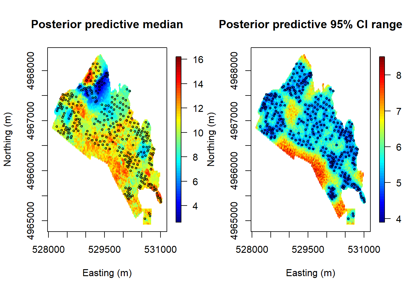

Finally, we’ll introduce several model comparison criteria.

The DIC criterion: The Deviance Information Criterion (DIC) is a generalization of the AIC, whose asymptotic justification is not appropriate for hierarchical (3 levels or more) models (see, e.g., Spiegelhalter et al. (2002)). Define the deviance statistic as \[D({\boldsymbol{\theta}}) = -\log p({\mathbf{y}}\,|\, {\boldsymbol{\theta}}) + 2\log h({\mathbf{y}}),\] where \(p({\mathbf{y}}\,|\, {\boldsymbol{\theta}})\) is the likelihood function and \(h({\mathbf{y}})\) is some standardizing function of the data alone (usually, \(h({\mathbf{y}})\) is set to be zero). The fitting performance of the model is evaluated by the posterior expectation of the deviance, that is \[\overline D = {\mathbb{E}}_{{\boldsymbol{\theta}}|{\mathbf{y}}}(D({\boldsymbol{\theta}})).\] The complexity of the model is summarized by the effective number of parameters \(p_D\). For Gaussian models, \(p_D\) can be defined as the difference between the expected deviance and the deviance evaluated at the posterior mean of \({\boldsymbol{\theta}}\), that is \[p_D = \overline D - D(\bar {\boldsymbol{\theta}}),\] where \(\bar {\boldsymbol{\theta}}= {\mathbb{E}}_{{\boldsymbol{\theta}}|{\mathbf{y}}}({\boldsymbol{\theta}})\). Then the DIC is defined by the summation of model fitting and model complexity, that is \[DIC = \overline D + p_D.\] So smaller values of \(DIC\) indicates a better model. Since \(\overline D\) and \(D({\boldsymbol{\theta}})\) can be obtained by posterior samples of \({\boldsymbol{\theta}}\), \(DIC\) is easy to be estimated with the MCMC estimation procedure.

Posterior predictive loss criterion: The criterion was proposed by A. E. Gelfand and Ghosh (1998). Assume we observe \({\mathbf{y}}= (y_1,...,y_n)^\top\). The criterion is defined by \[D_k = \frac{k}{k+1}G + P,\] where \(G = \sum_{i=1}^n (\mu_i - y_i)^2\) and \(P = \sum_{i=1}^n \sigma_i^2\) with \(\mu_i\) and \(\sigma_i^2\) representing the mean and variance of the posterior predictive distribution of \(Y\) given the observed data \({\mathbf{y}}\). \(G\) measures the fitting performance and \(P\) measures the variability. Their weights is adjusted by the integer \(k\). If \(k=\infty\), \(D_k = D_\infty = G+P.\)

The quantities \(\mu_i\) and \(\sigma_i^2\) can be easily obtained via samples of posterior predictive distributions.

Again, So smaller values of \(D_k\) indicates a better model.

Model assessment using hold out data: partition the data to training and test sets, fit the model with training sets, and evaluate model performance by measuring the mean square prediction errors of test data. Let \(y_{1,test},...,y_{m,test}\) be the test data and let \(\hat y_{1,test}, ..., \hat y_{m,test}\) be the posterior predicted mean. Then the mean square prediction error is defined by \[MSPR = \frac{1}{m} \sum_{i=1}^m (\hat y_{i,test} - y_{i,test})^2.\]

Now we apply the above model comparison criteria to the biomass Example above. We compare the non-spatial and spatial models.

#model comparison.
#First, we decide how many PCs should be included in the regression model
#We run non-spatial linear models and do model selection using AIC, BIC and PRESS

#All possible subsets selection
library(leaps)
b <- regsubsets(X.train, bio.train)
rs <- summary(b)
rs$outmat

##          PC1 PC2 PC3 PC4
## 1  ( 1 ) "*" " " " " " "
## 2  ( 1 ) "*" "*" " " " "
## 3  ( 1 ) "*" "*" "*" " "
## 4  ( 1 ) "*" "*" "*" "*"

#calculate adjusted R^2, AIC, corrected AIC, and BIC
om1 <- lm(bio.train~X.train[,1])
om2 <- lm(bio.train~X.train[,1]+X.train[,2])
om3 <- lm(bio.train~X.train[,1]+X.train[,2]+X.train[,3])
om4 <- lm(bio.train~X.train[,1]+X.train[,2]+X.train[,3]+X.train[,4])

om <- list(om1,om2,om3,om4)
n.train <- length(bio.train)

#number of parameters in each model in "om"
m <- 4
npar <- 3:7
#AIC
AIC<- sapply(1:m, function(x) round(extractAIC(om[[x]],k=2)[2],2))
AIC

## [1] 510.30 457.91 458.83 460.80

#BIC
BIC<- sapply(1:m, function(x) round(extractAIC(om[[x]],k=log(n.train))[2],2))
BIC

## [1] 517.94 469.38 474.12 479.92

#all possible subsets selection with PRESS
myPRESS <- function(x,y,indx){
  m1 <- lm(y~x[,indx])
  press <- sum((m1$residuals/(1-hatvalues(m1)))^2)
  return(press)
}

PRESS.indx <- matrix("", nrow = m, ncol = m)
colnames(PRESS.indx) <- c("PC1", "PC2", "PC3", "PC4")
PRESS <- rep(0,m)
for(i in 1:m)
{
  indx <- combn(m,i)
  n.indx <- ncol(indx)
  tmp <- sapply(1:n.indx, function(m) myPRESS(X.train, bio.train, indx[,m]))
  PRESS[i] <- round(min(tmp),2)
  PRESS.indx[i, indx[,which.min(tmp)]] <- "*"
}

PRESS.indx

##      PC1 PC2 PC3 PC4
## [1,] "*" ""  ""  "" 
## [2,] "*" "*" ""  "" 
## [3,] "*" "*" "*" "" 
## [4,] "*" "*" "*" "*"

PRESS

## [1] 1532.17 1312.69 1316.51 1323.70

#The best non-spatial model only includes the frist two principle 
#components of LiDAR Signal.

#the funtion "bayesLMRef" fits a simple Bayesian linear model with 
#reference (non-informative) priors
m2.nsp <- bayesLMRef(om2, n.samples)
burn.in <- 0.75*n.samples
m2.nsp.Diag <- spDiag(m2.nsp, start = burn.in, verbose = FALSE)
DIC.nsp <- m2.nsp.Diag$DIC
GP.nsp <- m2.nsp.Diag$GP

#MSPR
#prediction at s.test
pred.nsp <- spPredict(m2.nsp, start = burn.in, thin = 10,  
                      pred.covars = cbind(1,X.test[,1:2]))
#posterior predicted value and prediction interval
pred.nsp.summary <- apply(pred.nsp$p.y.predictive.samples, 1, 
                  function(x){quantile(x, prob=c(0.025,0.5,0.975))})
MSPR.nsp <- mean((pred.nsp.summary[2,]-bio.test)^2)


#Second, we add the spatial dependence structure and run Bayesian spatial models
#with the frist two principle components of LiDAR Signals.


#m2.sp first two PCs in X
p <- 3
priors <- list("beta.Norm"=list(rep(0,p), diag(1000000,p)),
               "phi.Unif"=c(-log(0.05)/max.dist, -log(0.01)/min.dist),
   "sigma.sq.IG"=c(2, fit.vario$cov.pars[1]),  "tau.sq.IG"=c(2, fit.vario$nugget))
m2.sp <- spLM(bio.train ~ X.train[,1:2], coords=as.matrix(s.train), starting=starting,
           tuning=tuning, priors=priors, cov.model="exponential",
           n.samples=n.samples, n.report=floor(n.samples/4))

## ----------------------------------------
##  General model description
## ----------------------------------------
## Model fit with 338 observations.
## 
## Number of covariates 3 (including intercept if specified).
## 
## Using the exponential spatial correlation model.
## 
## Number of MCMC samples 20000.
## 
## Priors and hyperpriors:
##  beta normal:
##  mu: 0.000   0.000   0.000   
##  cov:
##  1000000.000 0.000   0.000   
##  0.000   1000000.000 0.000   
##  0.000   0.000   1000000.000 
## 
##  sigma.sq IG hyperpriors shape=2.00000 and scale=2.11917
##  tau.sq IG hyperpriors shape=2.00000 and scale=1.68148
##  phi Unif hyperpriors a=0.00088 and b=0.15342
## -------------------------------------------------
##      Sampling
## -------------------------------------------------
## Sampled: 5000 of 20000, 25.00%
## Report interval Metrop. Acceptance rate: 28.62%
## Overall Metrop. Acceptance rate: 28.62%
## -------------------------------------------------
## Sampled: 10000 of 20000, 50.00%
## Report interval Metrop. Acceptance rate: 29.22%
## Overall Metrop. Acceptance rate: 28.92%
## -------------------------------------------------
## Sampled: 15000 of 20000, 75.00%
## Report interval Metrop. Acceptance rate: 30.10%
## Overall Metrop. Acceptance rate: 29.31%
## -------------------------------------------------
## Sampled: 20000 of 20000, 100.00%
## Report interval Metrop. Acceptance rate: 30.10%
## Overall Metrop. Acceptance rate: 29.51%
## -------------------------------------------------

burn.in <- 0.75*n.samples
m2.sp <- spRecover(m2.sp, start=burn.in, thin=10, verbose=FALSE)
m2.sp.Diag <- spDiag(m2.sp, verbose = FALSE)
DIC.sp <- m2.sp.Diag$DIC
GP.sp <- m2.sp.Diag$GP

#MSPR
#prediction at s.test
pred.sp <- spPredict(m2.sp, start = burn.in, thin = 10, pred.coords = s.test, 
                     pred.covars = cbind(1,X.test[,1:2]))

## ----------------------------------------
##  General model description
## ----------------------------------------
## Model fit with 338 observations.
## 
## Prediction at 113 locations.
## 
## Number of covariates 3 (including intercept if specified).
## 
## Using the exponential spatial correlation model.
## 
## -------------------------------------------------
##      Sampling
## -------------------------------------------------
## Sampled: 100 of 501, 19.76%
## Sampled: 200 of 501, 39.72%
## Sampled: 300 of 501, 59.68%
## Sampled: 400 of 501, 79.64%
## Sampled: 500 of 501, 99.60%

#posterior predicted value and prediction interval
pred.sp.summary<- apply(pred.sp$p.y.predictive.samples, 1, 
                        function(x){quantile(x, prob=c(0.025,0.5,0.975))})
MSPR.sp <- mean((pred.sp.summary[2,]-bio.test)^2)

print(cbind(DIC.nsp, DIC.sp))

##                  value    value
## bar.D       794.008944 302.1002
## D.bar.Omega 789.941399 130.4316
## pD            4.067545 171.6686
## DIC         798.076489 473.7689

print(cbind(GP.nsp, GP.sp))

##      value    value
## G 1288.807 147.2771
## P 1315.965 469.7822
## D 2604.772 617.0593

print(cbind(MSPR.nsp, MSPR.sp))

##      MSPR.nsp  MSPR.sp
## [1,] 3.434601 1.725311

#plots for comparing the prediction performance of spatial 
#vs non-spatial models
par(mfrow=c(1,2))
#plots comparing observed vs prediction of non-spatial models
a<-min(c(pred.nsp.summary, pred.sp.summary,bio.test))
b<-max(c(pred.nsp.summary, pred.sp.summary,bio.test))+8
n.test <- length(bio.test)
indx <- order(pred.nsp.summary[2,])
plot(c(1:n.test),bio.test[indx], typ="l",ylim=c(a,b),xlab=NA,ylab=NA,
     main = "non-spatial prediction")
#fitted quantiles 0.025,0.5,0.975
polygon(c(c(1:n.test),rev(c(1:n.test))),c(pred.nsp.summary[1, indx],
          rev(pred.nsp.summary[3, indx])),col="grey90",border=FALSE)
lines(c(1:n.test),bio.test[indx],lty=1,col="black")
lines(c(1:n.test),pred.nsp.summary[1, indx],lty=2,col="grey60")
lines(c(1:n.test),pred.nsp.summary[2, indx],lty=4,col="red")
lines(c(1:n.test),pred.nsp.summary[3, indx],lty=2,col="grey60")
legend(1,b,c("95% posterior band","predicted",
"obs"),lty=c(2,4,1),lwd=c(2.5,2.5),col=c("grey60","red","black"));

#plots comparing observed vs prediction of spatial models
n.test <- length(bio.test)
indx <- order(pred.sp.summary[2,])
plot(c(1:n.test),bio.test[indx], typ="l",ylim=c(a,b),xlab=NA,ylab=NA,
     main = "spatial prediction")
#fitted quantiles 0.025,0.5,0.975
polygon(c(c(1:n.test),rev(c(1:n.test))),c(pred.sp.summary[1, indx],
    rev(pred.sp.summary[3, indx])),col="grey90",border=FALSE)
lines(c(1:n.test),bio.test[indx],lty=1,col="black")
lines(c(1:n.test),pred.sp.summary[1, indx],lty=2,col="grey60")
lines(c(1:n.test),pred.sp.summary[2, indx],lty=4,col="red")
lines(c(1:n.test),pred.sp.summary[3, indx],lty=2,col="grey60")
legend(1,b,c("95% posterior band","predicted",
"obs"),lty=c(2,4,1),lwd=c(2.5,2.5),col=c("grey60","red","black"))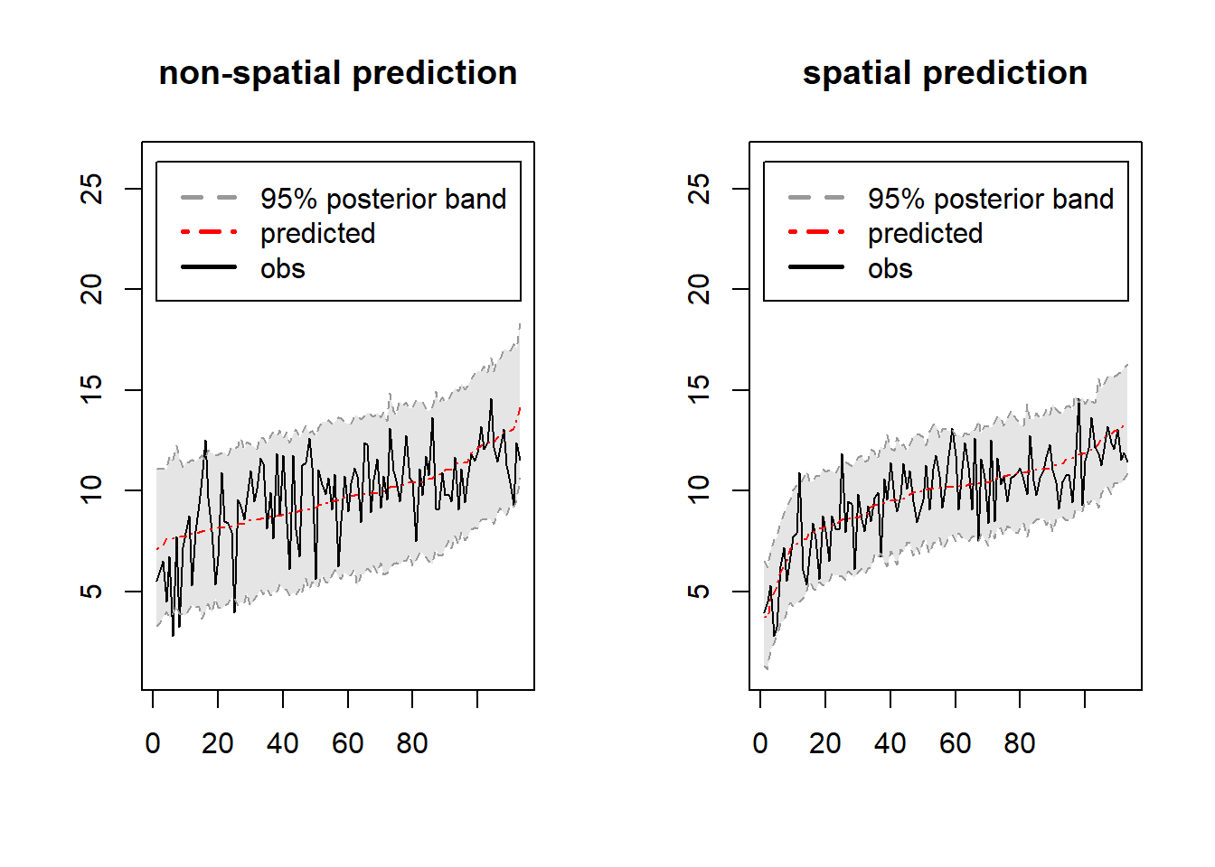

#The best model is spatial regression model with the frist two 
#principle components of LiDAR Signal.

3.5.3 Hierarchical Bayesian spatial models for non-Gaussian geostatistical data

Recall the hierarchical models for non-Gaussian geostatistical data. Adding priors for all parameters, we obtain Bayesian hierarchical models,

\[ \begin{align*} \text{data model: } &Y({\mathbf{s}})\, |\, \mu({\mathbf{s}}), \tilde {\boldsymbol{\theta}}\stackrel{ind.}{\sim} f(Y({\mathbf{s}})) \ \text{with}\ g(\mu({\mathbf{s}})) = {\mathbf{X}}({\mathbf{s}})^\top {\boldsymbol{\beta}}+ w({\mathbf{s}})\\ \text{process model: }& w({\mathbf{s}})\, |\, {\boldsymbol{\theta}}\sim Gaussian(0, C({\mathbf{h}};{\boldsymbol{\theta}}))\\ \text{parameter model: } & p({\boldsymbol{\beta}}, \tilde {\boldsymbol{\theta}}, {\boldsymbol{\theta}}), \end{align*} \] where \(\mu({\mathbf{s}}) := {\mathbb{E}}(Y({\mathbf{s}}) | w({\mathbf{s}}), {\boldsymbol{\beta}})\) is the mean of \(Y({\mathbf{s}})\) given \(w({\mathbf{s}})\) and \({\boldsymbol{\beta}}\), \(f(\cdot)\) is the density function of \(Y({\mathbf{s}})\) given \(\mu({\mathbf{s}})\) and \(\tilde {\boldsymbol{\theta}}\), \(C({\mathbf{h}}; {\boldsymbol{\theta}})\) is the spatial covariance function and \(p({\boldsymbol{\beta}}, \tilde {\boldsymbol{\theta}}, {\boldsymbol{\theta}})\) is the prior density of all parameters.

The prior specifications would be similar as those in Gaussian geostatistical data in the previous section.

The posterior distribution of the above Bayesian hierarchical model \[p({\boldsymbol{\beta}},{\boldsymbol{\theta}},\tilde {\boldsymbol{\theta}}, {\mathbf{w}}\,|\, {\mathbf{Y}}) \propto \prod_{i=1}^n f(Y({\mathbf{s}}_i) \,|\, w({\mathbf{s}}_i), {\mathbf{X}}({\mathbf{s}}_i), {\boldsymbol{\beta}}, \tilde {\boldsymbol{\theta}})p({\mathbf{w}}\,|\,{\boldsymbol{\theta}})p({\boldsymbol{\beta}})p(\tilde {\boldsymbol{\theta}})p({\boldsymbol{\theta}}).\] The above posterior distribution contains the latent variable \({\mathbf{w}}\) whose dimension is the number locations \(n\). Unfortunately, the latent variables \({\mathbf{w}}\) cannot be integrated out easily as done in Gaussian case. Hence, to get the Bayesian estimations for parameters \({\boldsymbol{\beta}}, {\boldsymbol{\theta}}, \tilde {\boldsymbol{\theta}}\), we have to sample from the posterior density \(p({\boldsymbol{\beta}},{\boldsymbol{\theta}},\tilde {\boldsymbol{\theta}}, {\mathbf{w}}\,|\, {\mathbf{Y}})\) which includes sampling the high dimension latent variable \({\mathbf{w}}\).

To predict \(Y\) at a new location \({\mathbf{s}}_0\), we can follow the similar method done in Gaussian case, that is we use composition sampling method to get the samples of \(Y({\mathbf{s}}_0)\) from its posterior predictive distribution, \[p(y({\mathbf{s}}_0)\,|\, {\mathbf{Y}}, {\mathbf{X}}({\mathbf{s}}_0)) = \int p(y({\mathbf{s}}_0) \,|\, {\mathbf{Y}}, \Theta, {\mathbf{X}}({\mathbf{s}}_0)) p(\Theta \,|\, {\mathbf{Y}})d\Theta,\] where \(\Theta = ({\boldsymbol{\beta}}, {\boldsymbol{\theta}}, \tilde {\boldsymbol{\theta}})\).

Here is a simulatoin study for Poisson spatial models without any predictors. Specifically, the density \(f(y) = \frac{e^{-\lambda({\mathbf{s}})}\lambda({\mathbf{s}})^k}{k!}\) and \(g(\mu({\mathbf{s}})) = \log(\lambda({\mathbf{s}})) = \beta_0 + w({\mathbf{s}})\).

rm(list=ls())
library(geoR)
library(geoRglm)
library(spBayes)
library(MASS)

#simulated Poisson spatial random field.
set.seed(1)
n <- 100
s <- cbind(runif(n,0,1), runif(n,0,1))
phi <- 6
sigmaSq <- 2
r <- exp(-iDist(s)*phi)
w <- mvrnorm(1,rep(0,n), sigmaSq*r)
beta0 <- 0.1
y <- rpois(n, exp(beta0+w))
## Visualising the data
plot(c(0, 1), c(0, 1), type="n", xlab="sx", ylab="sy")
text(s[,1], s[,2], format(y),cex=0.5)

#assume there is no spatial dependenc we might fit a simple non-spatial GLM using
pois.nonsp <- glm(y~1, family = "poisson")
beta.starting <- coefficients(pois.nonsp)
#tuning: Cholesky square root of the parameters' estimated covariances
beta.tuning <- t(chol(vcov(pois.nonsp)))

#MCMC chain1
n.batch <- 300
batch.length <- 50
n.samples <- n.batch * batch.length
dis <- iDist(s)
max.dis <- max(dis)
min.dis <- min(dis[dis!=0])
phi.a <- -log(0.05)/max.dis
phi.b <- -log(0.01)/min.dis
pois.sp.chain.1 <- spGLM(y ~ 1,family = "poisson",coords = s,
      starting = list(beta = beta.starting, phi = 0.5*phi.a + 0.5 *phi.b, sigma.sq = 1,w = 0),
      tuning = list(beta = 0.1, phi = 0.5, sigma.sq = 0.1,w = 0.1),
      priors = list("beta.Flat", phi.Unif = c(phi.a, phi.b), sigma.sq.IG = c(2, 1)),
      amcmc = list(n.batch = n.batch, batch.length=batch.length, accept.rate = 0.43),
      cov.model = "exponential")

## ----------------------------------------
##  General model description
## ----------------------------------------
## Model fit with 100 observations.
## 
## Number of covariates 1 (including intercept if specified).
## 
## Using the exponential spatial correlation model.
## 
## Number of MCMC samples 15000.
## 
## Priors and hyperpriors:
##  beta flat.
## 
##  sigma.sq IG hyperpriors shape=2.00000 and scale=1.00000
## 
##  phi Unif hyperpriors a=2.44795 and b=472.77259
## 
## Adaptive Metropolis with target acceptance rate: 43.0
## -------------------------------------------------
##      Sampling
## -------------------------------------------------
## Batch: 100 of 300, 33.33%
##  parameter   acceptance  tuning
##  beta[0]     44.0        0.15068
##  sigma.sq    54.0        0.27456
##  phi     36.0        0.68171
## -------------------------------------------------
## Batch: 200 of 300, 66.67%
##  parameter   acceptance  tuning
##  beta[0]     42.0        0.15068
##  sigma.sq    38.0        0.32220
##  phi     24.0        0.70953
## -------------------------------------------------
## Sampled: 15000 of 15000, 100.00%
## -------------------------------------------------

#MCMC chain2
pois.sp.chain.2 <- spGLM(y ~ 1,family = "poisson",coords = s,
starting = list(beta = beta.starting/4, phi = 0.25*phi.a + 0.75 *phi.b, sigma.sq = 0.5,w = 1),
tuning = list(beta = 0.1, phi = 0.5, sigma.sq = 0.1,w = 0.1),
priors = list("beta.Flat", phi.Unif = c(phi.a, phi.b), sigma.sq.IG = c(2, 1)),
amcmc = list(n.batch = n.batch, batch.length=batch.length, accept.rate = 0.43),
cov.model = "exponential")

## ----------------------------------------
##  General model description
## ----------------------------------------
## Model fit with 100 observations.
## 
## Number of covariates 1 (including intercept if specified).
## 
## Using the exponential spatial correlation model.
## 
## Number of MCMC samples 15000.
## 
## Priors and hyperpriors:
##  beta flat.
## 
##  sigma.sq IG hyperpriors shape=2.00000 and scale=1.00000
## 
##  phi Unif hyperpriors a=2.44795 and b=472.77259
## 
## Adaptive Metropolis with target acceptance rate: 43.0
## -------------------------------------------------
##      Sampling
## -------------------------------------------------
## Batch: 100 of 300, 33.33%
##  parameter   acceptance  tuning
##  beta[0]     40.0        0.13364
##  sigma.sq    52.0        0.25857
##  phi     54.0        0.65498
## -------------------------------------------------
## Batch: 200 of 300, 66.67%
##  parameter   acceptance  tuning
##  beta[0]     20.0        0.15373
##  sigma.sq    32.0        0.35609
##  phi     50.0        0.65498
## -------------------------------------------------
## Sampled: 15000 of 15000, 100.00%
## -------------------------------------------------

#MCMC chain3
pois.sp.chain.3 <- spGLM(y ~ 1,family = "poisson",coords = s,
starting = list(beta = beta.starting*4, phi = 0.75*phi.a + 0.25 *phi.b, sigma.sq = 1.5,w = 2),
tuning = list(beta = 0.1, phi = 0.5, sigma.sq = 0.1,w = 0.1),
priors = list("beta.Flat", phi.Unif = c(phi.a, phi.b), sigma.sq.IG = c(2, 1)),
amcmc = list(n.batch = n.batch, batch.length=batch.length, accept.rate = 0.43),
cov.model = "exponential")

## ----------------------------------------
##  General model description
## ----------------------------------------
## Model fit with 100 observations.
## 
## Number of covariates 1 (including intercept if specified).
## 
## Using the exponential spatial correlation model.
## 
## Number of MCMC samples 15000.
## 
## Priors and hyperpriors:
##  beta flat.
## 
##  sigma.sq IG hyperpriors shape=2.00000 and scale=1.00000
## 
##  phi Unif hyperpriors a=2.44795 and b=472.77259
## 
## Adaptive Metropolis with target acceptance rate: 43.0
## -------------------------------------------------
##      Sampling
## -------------------------------------------------
## Batch: 100 of 300, 33.33%
##  parameter   acceptance  tuning
##  beta[0]     58.0        0.13634
##  sigma.sq    50.0        0.26379
##  phi     54.0        0.62930
## -------------------------------------------------
## Batch: 200 of 300, 66.67%
##  parameter   acceptance  tuning
##  beta[0]     40.0        0.14477
##  sigma.sq    40.0        0.32220
##  phi     58.0        0.61684
## -------------------------------------------------
## Sampled: 15000 of 15000, 100.00%
## -------------------------------------------------

#plot: MCMC chains trace
samps <- mcmc.list(pois.sp.chain.1$p.beta.theta.samples,
                   pois.sp.chain.2$p.beta.theta.samples,
                   pois.sp.chain.3$p.beta.theta.samples)

plot(samps)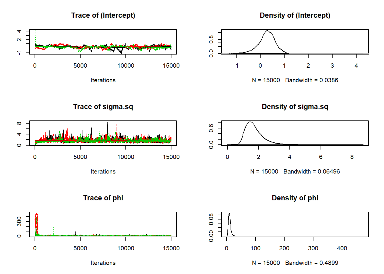

#Diagnostics Of MCMC converges:
#"potential scale reduction factor" for each parameter obtained by "gelman.diag"
#approximate convergence is diagnosed when the upper confidence limit is close to 1. 
print(gelman.diag(samps))

## Potential scale reduction factors:
## 
##             Point est. Upper C.I.
## (Intercept)       1.09       1.26
## sigma.sq          1.02       1.05
## phi               1.01       1.02
## 
## Multivariate psrf
## 
## 1.06

#"gelman.plot" plot the Gelman and Rubin's shrink factor versus MCMC samples;
#covergence is diagnosed wehn the upper confidence limit remains close to 1.
gelman.plot(samps)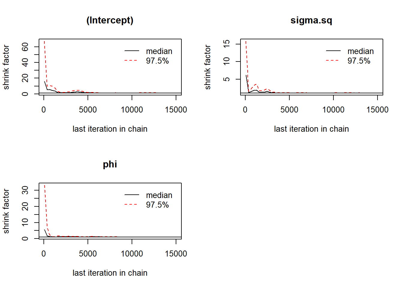

#we pick the first 10,000 samples as burn-in.  
burn.in <- 10000
print(round(summary(window(samps, start = burn.in))$quantiles[,c(3,1,5)], 2))

##              50%  2.5% 97.5%
## (Intercept) 0.29 -0.40  0.84
## sigma.sq    1.56  0.95  2.87
## phi         9.48  4.29 19.79

pred.coords <- as.matrix(expand.grid(seq(0.01, 0.99,length.out = 20),
                seq(0.01, 0.99, length.out = 20)))
pred.covars <- as.matrix(rep(1, nrow(pred.coords)))
pois.pred <- spPredict(pois.sp.chain.1, start = 10000, thin = 10,
            pred.coords = pred.coords, pred.covars = pred.covars)

## -------------------------------------------------
##      Starting prediction
## -------------------------------------------------
## Sampled: 100 of 501, 19.96%
## Sampled: 200 of 501, 39.92%
## Sampled: 300 of 501, 59.88%
## Sampled: 400 of 501, 79.84%
## Sampled: 500 of 501, 99.80%

y.pred <- apply(pois.pred$p.y.predictive.samples,1,median)

par(mfrow = c(1, 2))
surf <- mba.surf(cbind(s, y), no.X = 100, no.Y = 100, extend = TRUE)$xyz.est
image.plot(surf, main = "Observed counts")
points(s)
surf <- mba.surf(cbind(pred.coords, y.pred), no.X = 100, no.Y = 100, extend = TRUE)$xyz.est
image.plot(surf, main = "Predicted counts")
points(pred.coords, pch = "x", cex = 1)
points(s, pch = 19, cex = 1)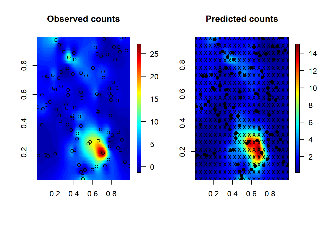

References

Cressie, N.A.C. 1993. Statistics for spatial data, 2nd ed. New York: Jone Wiley & Sons.

Diggle, Peter J, JA Tawn, and RA Moyeed. 1998. “Model-Based Geostatistics.” Journal of the Royal Statistical Society: Series C (Applied Statistics) 47 (3). Wiley Online Library: 299–350.

Gelfand, A., P. Diggle, M. Fuentes, and P. Guttorp. 2010. Handbook of spatial statistics. CRC press.

Gelfand, Alan E, and Sujit K Ghosh. 1998. “Model Choice: A Minimum Posterior Predictive Loss Approach.” Biometrika 85 (1). Oxford University Press: 1–11.

Gelman, Andrew, John B Carlin, Hal S Stern, David B Dunson, Aki Vehtari, and Donald B Rubin. 2014. Bayesian Data Analysis. Vol. 2. CRC press Boca Raton, FL.

Lahiri, Soumendra Nath, Yoondong Lee, and Noel Cressie. 2002. “On Asymptotic Distribution and Asymptotic Efficiency of Least Squares Estimators of Spatial Variogram Parameters.” Journal of Statistical Planning and Inference 103 (1). Elsevier: 65–85.

Ren, Qian, and Sudipto Banerjee. 2013. “Hierarchical Factor Models for Large Spatially Misaligned Data: A Low-Rank Predictive Process Approach.” Biometrics 69 (1). Wiley Online Library: 19–30.

Schabenberger, Oliver, and Carol A Gotway. 2017. Statistical Methods for Spatial Data Analysis. CRC press.

Spiegelhalter, David J, Nicola G Best, Bradley P Carlin, and Angelika Van Der Linde. 2002. “Bayesian Measures of Model Complexity and Fit.” Journal of the Royal Statistical Society: Series B (Statistical Methodology) 64 (4). Wiley Online Library: 583–639.